5 Handling date-time data with `lubridate`

## 
## Attaching package: 'lubridate'

## The following objects are masked from 'package:base':
## 
##     date, intersect, setdiff, union

Date-time data can be complex to handle in R. Classic R commands for date-times are generally unintuitive and vary depending on the date-time object being used. the lubridate package makes it easier to handle date-times in R and handle many tasks classic R functions cannot handle.

We will cover some useful commands within the package but do consult the lubridate cheat sheet below for a series of useful commands.

Lubridate cheat sheet

5.1 Creating date/times

There are three types of date/time data that refer to an instant in time:

A date. Tibbles print this as <date>
A time within a day. Tibbles print this as <time>
A date-time is a date plus a time: it uniquely identifies an instant in time. Tibbles print this as <dttm>.

You should always use the simplest possible data type for what you need.

There are three ways you are likely to create a date/time:

From a string
From date/time components
From an existing date/time object

These can be created as follows.

5.1.1 From strings

We can convert a string to a date/time object using functions within lubridate. These functions automatically work out the format once you specify the order of the component. To use them, identify the order in which year, month and day appear in your dates, then arrange “y”, “m”, and “d” in the same order. This gives you the name of the function you need to call. For example:

ymd("2022-08-02")

## [1] "2022-08-02"

mdy("August 2nd, 2022")

## [1] "2022-08-02"

dmy("02-Aug-2022")

## [1] "2022-08-02"

These functions also take unquoted numbers. This is the most concise way to create a single date/time object.

ymd(20220802)

## [1] "2022-08-02"

To create a date-time, add an underscore to the previous functions and one or more of “h”, “m” and “s” to the name of the function

ymd_hms("2022-08-02 13:05:02")

## [1] "2022-08-02 13:05:02 UTC"

mdy_hm("08/02/2022 13:05")

## [1] "2022-08-02 13:05:00 UTC"

You can also force the creation of a date-time from a date by supplying a timezone

ymd(20220802,tz="UTC")

## [1] "2022-08-02 UTC"

5.1.2 From individual components

Instead of a string, you sometimes may have individual components of the date-time spread across multiple columns. Looking at data provided within the nycflights13 library, we see

library(nycflights13)
library(tidyverse)

flights %>%
  select(year,month,day,hour,minute)

## # A tibble: 336,776 × 5
##     year month   day  hour minute
##    <int> <int> <int> <dbl>  <dbl>
##  1  2013     1     1     5     15
##  2  2013     1     1     5     29
##  3  2013     1     1     5     40
##  4  2013     1     1     5     45
##  5  2013     1     1     6      0
##  6  2013     1     1     5     58
##  7  2013     1     1     6      0
##  8  2013     1     1     6      0
##  9  2013     1     1     6      0
## 10  2013     1     1     6      0
## # … with 336,766 more rows

To create a date/time for this data, we can use make_date() for dates, or make_datetime() for date-times:

flights <- flights %>%
  select(year,month,day,hour,minute) %>%
  mutate(departure_time=make_datetime(year,month,day,hour,minute))

5.1.3 From existing types

You may wish to switch between a date-time and a date. This can be done using as_datetime() and as_date()

as_datetime(today())

## [1] "2022-08-02 UTC"

as_date(now())

## [1] "2022-08-02"

5.2 Date-time Components

Here, we will look at functions which can let us access certain components of a date-time object.

You can obtain certain parts of a date with functions like year(), month(), mday() (day of month), yday() (day of year), hour(), minute() and second().

date_time <- ymd_hms("2021-12-25,09:10:25")

year(date_time)

## [1] 2021

month(date_time)

## [1] 12

mday(date_time)

## [1] 25

yday(date_time)

## [1] 359

For month() and wday(), you can set label=TRUE to return the abbreviated name of the month or day of the week. Set abbr=FALSE to return the full name.

month(date_time,label=TRUE)

## [1] Dec
## 12 Levels: Jan < Feb < Mar < Apr < May < Jun < Jul < Aug < Sep < ... < Dec

wday(date_time,label=TRUE,abbr=FALSE)

## [1] Saturday
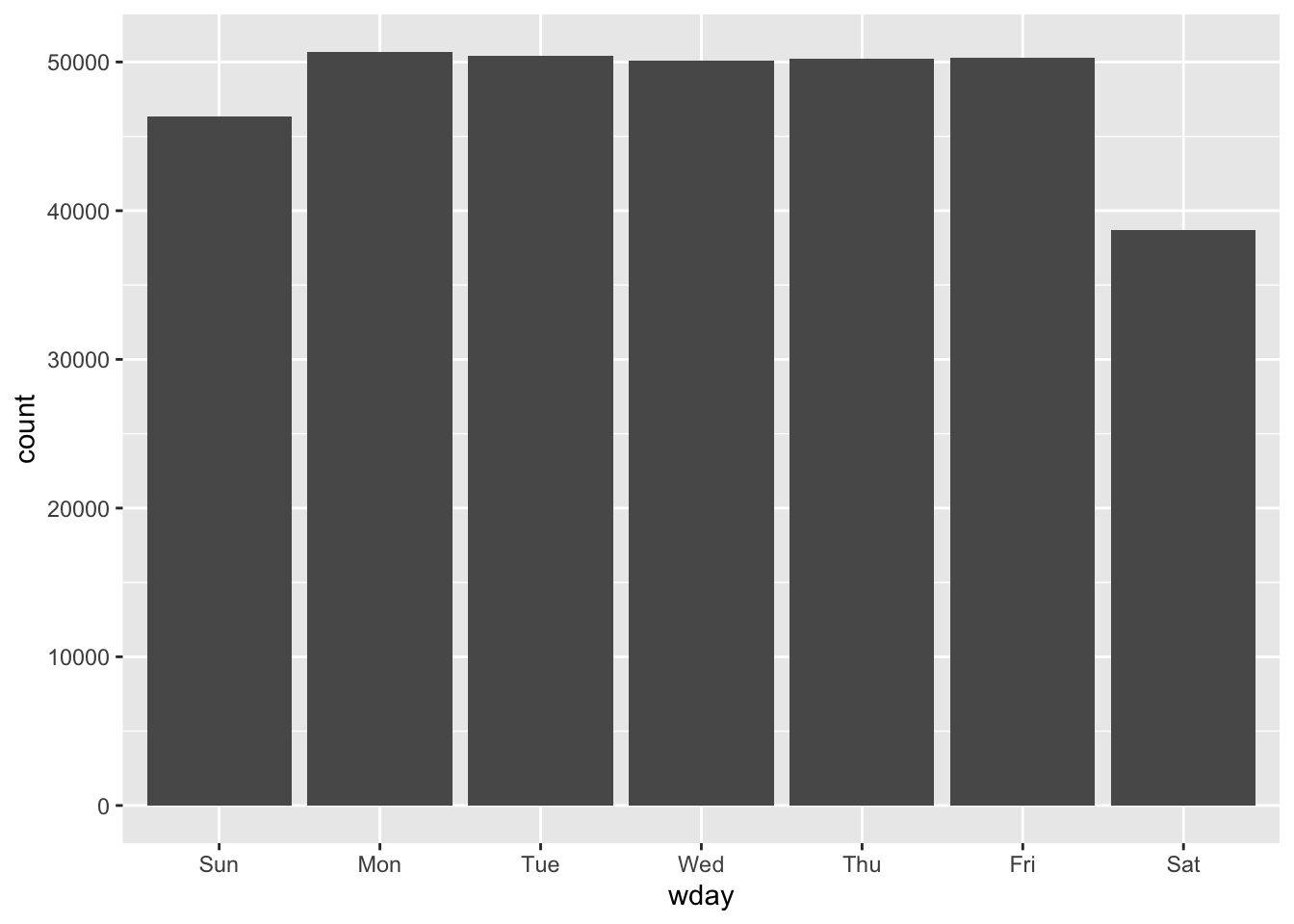
## 7 Levels: Sunday < Monday < Tuesday < Wednesday < Thursday < ... < Saturday

We can use wday() to see that more flights depart during the week than on the weekend

flights %>% 
  mutate(wday = wday(departure_time, label = TRUE)) %>% 
  ggplot(aes(x = wday)) +
    geom_bar()

5.2.1 Time Spans

Now we will look at how arithmetic with dates works, including subtraction, addition and division. We will explore the following three classes:

durations, which represent an exact number of seconds
periods, which represent units like weeks and months
intervals, which represent a start and end point

5.2.2 Durations

We can find out the duration (given in seconds) using the as.duration() function as shown below

# How old is Craig?
c_age <- today() - ymd(19910502)
as.duration(c_age)

## [1] "986256000s (~31.25 years)"

Durations also come with some useful additional functions shown below

dseconds(10)

## [1] "10s"

dminutes(60)

## [1] "3600s (~1 hours)"

dhours(30)

## [1] "108000s (~1.25 days)"

ddays(c(4,15))

## [1] "345600s (~4 days)"      "1296000s (~2.14 weeks)"

dweeks(1:4)

## [1] "604800s (~1 weeks)"  "1209600s (~2 weeks)" "1814400s (~3 weeks)"
## [4] "2419200s (~4 weeks)"

dyears(2)

## [1] "63115200s (~2 years)"

We can also add and multiply durations

3*dmonths(5)

## [1] "39447000s (~1.25 years)"

dyears(3) + dweeks(14) +dhours(6)

## [1] "103161600s (~3.27 years)"

5.2.3 Periods

Periods are time spans, but don’t have a fixed length in seconds, and work more as “human” times, like days and weeks.

today() + days(1)

## [1] "2022-08-03"

Like durations, periods can be constructed using well named constructor functions.

seconds(15)

## [1] "15S"

minutes(10)

## [1] "10M 0S"

hours(30)

## [1] "30H 0M 0S"

days(c(2,5))

## [1] "2d 0H 0M 0S" "5d 0H 0M 0S"

months(2:5)

## [1] "2m 0d 0H 0M 0S" "3m 0d 0H 0M 0S" "4m 0d 0H 0M 0S" "5m 0d 0H 0M 0S"

weeks(3)

## [1] "21d 0H 0M 0S"

years(1)

## [1] "1y 0m 0d 0H 0M 0S"

Like durations, we can add and multiply periods

3*(months(4) + days(12))

## [1] "12m 36d 0H 0M 0S"

days(25) + hours(16) + minutes(12)

## [1] "25d 16H 12M 0S"

5.2.4 Intervals

An interval is a duration with a starting point, this makes it precise so you can determine exactly how long it is:

next_year <- today() + years(1)
(today() %--% next_year)/ddays(1)

## [1] 365

To find out how many periods fall into an interval, you need to use integer division %/%

4 Creating Graphics with ggplot2

6 Producing maps for plotting

5 Handling date-time data with lubridate