5 Uygulama - 1
Bu bölümde iki grubun ortalama farkına dayalı etki büyüklüğü değerleri kullanılarak meta analiz çalışması yapılmıştır. Bu çalışmada Hedge g, MD (standartlaştırılmamış ortalama farkı ile etki büyüklüğü), Cohen’ s d ve standart hatalar hesaplanmıştır.
library(readxl)

# Excel dosyasını oku
data <- read_excel("s176.xlsx")

# Veri setini kontrol et
head(data)
## # A tibble: 6 × 6
## mean_exp sd_exp n_exp mean_control sd_control n_control
## <dbl> <dbl> <dbl> <dbl> <dbl> <dbl>
## 1 70.7 15.5 27 56.3 18.6 73
## 2 59.4 9.8 15 41.7 90.4 45
## 3 33.7 25.2 31 26.6 20.3 42
## 4 3.69 2.83 29 3.07 2.2 30
## 5 5.17 2.85 30 3.07 2.2 30
## 6 6.04 2.83 18 6.06 2.76 21# Deney ve kontrol gruplarına ait veriler
mean_exp <- data$mean_exp # Deney grubunun aritmetik ortalaması
mean_control <- data$mean_control # Kontrol grubunun aritmetik ortalaması
sd_exp <- data$sd_exp # Deney grubunun standart sapması
sd_control <- data$sd_control # Kontrol grubunun standart sapması
n_exp <- data$n_exp # Deney grubunun örneklem büyüklüğü
n_control <- data$n_control # Kontrol grubunun örneklem büyüklüğü
# 1. Birleşik Standart Sapma (Pooled Standard Deviation)
pooled_sd <- sqrt(((n_exp - 1) * sd_exp^2 + (n_control - 1) * sd_control^2) / (n_exp + n_control - 2))
# 2. Standartlaştırılmış Ortalama Fark (Cohen's d)
d <- (mean_exp - mean_control) / pooled_sd
# 3. Cohen's d için Standart Hata (SE_d)
SE_d <- sqrt((n_exp + n_control) / (n_exp * n_control) + (d^2 / (2 * (n_exp + n_control))))
# 4. Hedges's g hesaplama
g <- d * (1 - (3 / (4 * (n_exp + n_control - 2) - 1)))
# 5. Hedges's g için Standart Hata (SE_g) fonksiyonu
SE_g <- function(SE_d, n_exp, n_control) {
SE_g <- SE_d * (1 - (3 / (4 * (n_exp + n_control) - 9)))
return(SE_g)
}
SE_g_values <- SE_g(SE_d, n_exp, n_control)
# 6. Standartlaştırılmamış Ortalama Farkı (MD)
MD <- mean_exp - mean_control
# 7. MD'nin Standart Hatası (SE_MD)
SE_MD <- sqrt((sd_exp^2 / n_exp) + (sd_control^2 / n_control))
# Sonuçları yazdır
cat("Cohen's d değerleri: \n")## Cohen's d değerleri:## [1] 0.810350527 0.224885979 0.316112340 0.245140635 0.824878355
## [6] -0.007162349 1.450999155 1.644585669 0.930429782 1.264409058
## [11] 0.759959555 -1.973492204 0.145402658 -0.009238950 0.472986506
## [16] 0.577909478 -0.052614517## Cohen's d için Standart Hata değerleri:## [1] 0.2324199 0.2988484 0.2382268 0.2613912 0.2689551 0.3212091 0.2497730
## [8] 0.2701259 0.3843978 0.3999735 0.2989136 0.4608740 0.1533578 0.5000027
## [15] 0.2058997 0.2112821 0.1550166## Hedges's g değerleri:## [1] 0.804133004 0.221965382 0.312761326 0.241900890 0.814165649
## [6] -0.007016178 1.437180115 1.627394878 0.905283031 1.230235840
## [11] 0.747501202 -1.916011848 0.144756424 -0.008735008 0.469242550
## [16] 0.573185422 -0.052374997## Hedges's g için Standart Hata değerleri:## [1] 0.2306366 0.2949672 0.2357015 0.2579367 0.2654622 0.3146538 0.2473942
## [8] 0.2673023 0.3740087 0.3891635 0.2940134 0.4474505 0.1526762 0.4727298
## [15] 0.2042699 0.2095550 0.1543109## Standartlaştırılmamış Ortalama Farkı (MD) değerleri:## [1] 14.44 17.74 7.11 0.62 2.10 -0.02 18.97 23.06 1.85 1.95
## [11] 2.83 -20.72 3.75 -0.40 5.37 11.47 -0.53## MD için Standart Hata değerleri (SE_MD):## [1] 3.6946066 13.7115361 5.5007047 0.6614396 0.6573305 0.8987112
## [7] 2.9205963 3.4603797 0.7260349 0.5631400 1.0749922 3.9683075
## [13] 3.9399131 21.6474805 2.3003483 4.0235682 1.5589856# Çalışma bazında sonuçları görmek isterseniz:
results <- data.frame(
study = 1:nrow(data),
mean_exp = mean_exp,
mean_control = mean_control,
pooled_sd = pooled_sd,
d = d,
SE_d = SE_d,
g = g,
SE_g = SE_g_values,
MD = MD,
SE_MD = SE_MD
)
# Sonuçları görüntüle
print(results)## study mean_exp mean_control pooled_sd d SE_d g
## 1 1 70.71 56.27 17.819449 0.810350527 0.2324199 0.804133004
## 2 2 59.40 41.66 78.884420 0.224885979 0.2988484 0.221965382
## 3 3 33.71 26.60 22.492004 0.316112340 0.2382268 0.312761326
## 4 4 3.69 3.07 2.529160 0.245140635 0.2613912 0.241900890
## 5 5 5.17 3.07 2.545830 0.824878355 0.2689551 0.814165649
## 6 6 6.04 6.06 2.792380 -0.007162349 0.3212091 -0.007016178
## 7 7 94.58 75.61 13.073750 1.450999155 0.2497730 1.437180115
## 8 8 98.67 75.61 14.021769 1.644585669 0.2701259 1.627394878
## 9 9 7.45 5.60 1.988328 0.930429782 0.3843978 0.905283031
## 10 10 4.40 2.45 1.542222 1.264409058 0.3999735 1.230235840
## 11 11 19.12 16.29 3.723882 0.759959555 0.2989136 0.747501202
## 12 12 45.71 66.43 10.499155 -1.973492204 0.4608740 -1.916011848
## 13 13 50.50 46.75 25.790450 0.145402658 0.1533578 0.144756424
## 14 14 52.88 53.28 43.294961 -0.009238950 0.5000027 -0.008735008
## 15 15 73.43 68.06 11.353389 0.472986506 0.2058997 0.469242550
## 16 16 55.91 44.44 19.847399 0.577909478 0.2112821 0.573185422
## 17 17 20.94 21.47 10.073266 -0.052614517 0.1550166 -0.052374997
## SE_g MD SE_MD
## 1 0.2306366 14.44 3.6946066
## 2 0.2949672 17.74 13.7115361
## 3 0.2357015 7.11 5.5007047
## 4 0.2579367 0.62 0.6614396
## 5 0.2654622 2.10 0.6573305
## 6 0.3146538 -0.02 0.8987112
## 7 0.2473942 18.97 2.9205963
## 8 0.2673023 23.06 3.4603797
## 9 0.3740087 1.85 0.7260349
## 10 0.3891635 1.95 0.5631400
## 11 0.2940134 2.83 1.0749922
## 12 0.4474505 -20.72 3.9683075
## 13 0.1526762 3.75 3.9399131
## 14 0.4727298 -0.40 21.6474805
## 15 0.2042699 5.37 2.3003483
## 16 0.2095550 11.47 4.0235682
## 17 0.1543109 -0.53 1.5589856Bu kısımda Hedge’s g, standart hata, varyans değeri, güven aralığı, z değeri ve p değeri hesaplanmıştır. Bu değerler orman garfiği kullanılarak gösterilmiştir.
library(readxl)
library(ggplot2)

# Excel dosyasını oku
data <- read_excel("s176.xlsx")

# Veri setini kontrol et
head(data)
## # A tibble: 6 × 6
## mean_exp sd_exp n_exp mean_control sd_control n_control
## <dbl> <dbl> <dbl> <dbl> <dbl> <dbl>
## 1 70.7 15.5 27 56.3 18.6 73
## 2 59.4 9.8 15 41.7 90.4 45
## 3 33.7 25.2 31 26.6 20.3 42
## 4 3.69 2.83 29 3.07 2.2 30
## 5 5.17 2.85 30 3.07 2.2 30
## 6 6.04 2.83 18 6.06 2.76 21# Deney ve kontrol gruplarına ait veriler
mean_exp <- data$mean_exp # Deney grubunun aritmetik ortalaması
mean_control <- data$mean_control # Kontrol grubunun aritmetik ortalaması
sd_exp <- data$sd_exp # Deney grubunun standart sapması
sd_control <- data$sd_control # Kontrol grubunun standart sapması
n_exp <- data$n_exp # Deney grubunun örneklem büyüklüğü
n_control <- data$n_control # Kontrol grubunun örneklem büyüklüğü
# 1. Birleşik Standart Sapma (Pooled Standard Deviation)
pooled_sd <- sqrt(((n_exp - 1) * sd_exp^2 + (n_control - 1) * sd_control^2) / (n_exp + n_control - 2))
# 2. Hedges's g hesaplama
g <- (mean_exp - mean_control) / pooled_sd * (1 - (3 / (4 * (n_exp + n_control - 2) - 1)))
# 3. Hedges's g için Standart Hata (SE_g)
SE_g <- sqrt((n_exp + n_control) / (n_exp * n_control) + (g^2 / (2 * (n_exp + n_control)))) * (1 - (3 / (4 * (n_exp + n_control) - 9)))
# 4. Varyans (Variance of g)
var_g <- SE_g^2
# 5. Güven Aralığı (95% CI)
z_critical <- 1.96 # 95% güven aralığı için
lower_ci <- g - z_critical * SE_g
upper_ci <- g + z_critical * SE_g
# 6. Z-değeri (Z-value)
z_value <- g / SE_g
# 7. P-değeri (P-value)
p_value <- 2 * (1 - pnorm(abs(z_value)))
# Sonuçları yazdır
cat("Hedges's g değerleri: \n")## Hedges's g değerleri:## [1] 0.804133004 0.221965382 0.312761326 0.241900890 0.814165649
## [6] -0.007016178 1.437180115 1.627394878 0.905283031 1.230235840
## [11] 0.747501202 -1.916011848 0.144756424 -0.008735008 0.469242550
## [16] 0.573185422 -0.052374997## Hedges's g için Standart Hata (SE_g) değerleri:## [1] 0.2305295 0.2949492 0.2356715 0.2579115 0.2651936 0.3146537 0.2469052
## [8] 0.2666053 0.3730337 0.3874314 0.2936914 0.4432254 0.1526744 0.4727295
## [15] 0.2042260 0.2094871 0.1543107## Hedges's g Varyansı (var_g):## [1] 0.05314383 0.08699506 0.05554104 0.06651832 0.07032764 0.09900697
## [7] 0.06096218 0.07107838 0.13915413 0.15010312 0.08625462 0.19644879
## [13] 0.02330948 0.22347321 0.04170828 0.04388486 0.02381179## Hedges's g için Güven Aralıkları (95% CI):## Lower Upper
## 1 0.35229528 1.2559707
## 2 -0.35613513 0.8000659
## 3 -0.14915477 0.7746774
## 4 -0.26360556 0.7474073
## 5 0.29438620 1.3339451
## 6 -0.62373750 0.6097051
## 7 0.95324593 1.9211143
## 8 1.10484852 2.1499412
## 9 0.17413700 1.6364291
## 10 0.47087022 1.9896015
## 11 0.17186613 1.3231363
## 12 -2.78473372 -1.0472900
## 13 -0.15448542 0.4439983
## 14 -0.93528488 0.9178149
## 15 0.06895951 0.8695256
## 16 0.16259063 0.9837802
## 17 -0.35482395 0.2500740## Z-değerleri (z-value):## [1] 3.48820075 0.75255451 1.32710725 0.93792224 3.07008034 -0.02229809
## [7] 5.82077712 6.10413590 2.42681307 3.17536398 2.54519301 -4.32288326
## [13] 0.94813810 -0.01847781 2.29766265 2.73613659 -0.33941263## P-değerleri (p-value):## [1] 4.862828e-04 4.517177e-01 1.844732e-01 3.482844e-01 2.140012e-03
## [6] 9.822102e-01 5.857464e-09 1.033583e-09 1.523210e-02 1.496487e-03
## [11] 1.092174e-02 1.540032e-05 3.430592e-01 9.852577e-01 2.158100e-02
## [16] 6.216522e-03 7.342989e-01# Çalışma bazında sonuçları görmek isterseniz:
results <- data.frame(
study = 1:nrow(data),
mean_exp = mean_exp,
mean_control = mean_control,
pooled_sd = pooled_sd,
g = g,
SE_g = SE_g,
var_g = var_g,
lower_ci = lower_ci,
upper_ci = upper_ci,
z_value = z_value,
p_value = p_value
)
# Sonuçları görüntüle
print(results)## study mean_exp mean_control pooled_sd g SE_g var_g
## 1 1 70.71 56.27 17.819449 0.804133004 0.2305295 0.05314383
## 2 2 59.40 41.66 78.884420 0.221965382 0.2949492 0.08699506
## 3 3 33.71 26.60 22.492004 0.312761326 0.2356715 0.05554104
## 4 4 3.69 3.07 2.529160 0.241900890 0.2579115 0.06651832
## 5 5 5.17 3.07 2.545830 0.814165649 0.2651936 0.07032764
## 6 6 6.04 6.06 2.792380 -0.007016178 0.3146537 0.09900697
## 7 7 94.58 75.61 13.073750 1.437180115 0.2469052 0.06096218
## 8 8 98.67 75.61 14.021769 1.627394878 0.2666053 0.07107838
## 9 9 7.45 5.60 1.988328 0.905283031 0.3730337 0.13915413
## 10 10 4.40 2.45 1.542222 1.230235840 0.3874314 0.15010312
## 11 11 19.12 16.29 3.723882 0.747501202 0.2936914 0.08625462
## 12 12 45.71 66.43 10.499155 -1.916011848 0.4432254 0.19644879
## 13 13 50.50 46.75 25.790450 0.144756424 0.1526744 0.02330948
## 14 14 52.88 53.28 43.294961 -0.008735008 0.4727295 0.22347321
## 15 15 73.43 68.06 11.353389 0.469242550 0.2042260 0.04170828
## 16 16 55.91 44.44 19.847399 0.573185422 0.2094871 0.04388486
## 17 17 20.94 21.47 10.073266 -0.052374997 0.1543107 0.02381179
## lower_ci upper_ci z_value p_value
## 1 0.35229528 1.2559707 3.48820075 4.862828e-04
## 2 -0.35613513 0.8000659 0.75255451 4.517177e-01
## 3 -0.14915477 0.7746774 1.32710725 1.844732e-01
## 4 -0.26360556 0.7474073 0.93792224 3.482844e-01
## 5 0.29438620 1.3339451 3.07008034 2.140012e-03
## 6 -0.62373750 0.6097051 -0.02229809 9.822102e-01
## 7 0.95324593 1.9211143 5.82077712 5.857464e-09
## 8 1.10484852 2.1499412 6.10413590 1.033583e-09
## 9 0.17413700 1.6364291 2.42681307 1.523210e-02
## 10 0.47087022 1.9896015 3.17536398 1.496487e-03
## 11 0.17186613 1.3231363 2.54519301 1.092174e-02
## 12 -2.78473372 -1.0472900 -4.32288326 1.540032e-05
## 13 -0.15448542 0.4439983 0.94813810 3.430592e-01
## 14 -0.93528488 0.9178149 -0.01847781 9.852577e-01
## 15 0.06895951 0.8695256 2.29766265 2.158100e-02
## 16 0.16259063 0.9837802 2.73613659 6.216522e-03
## 17 -0.35482395 0.2500740 -0.33941263 7.342989e-01forest_plot <- ggplot(results, aes(x = g, y = study)) +
geom_point(shape = 15, size = 3, color = "blue") + # Hedges's g noktaları
geom_errorbarh(aes(xmin = lower_ci, xmax = upper_ci), height = 0.2, color = "red") + # %95 CI yatay hata çubukları
geom_vline(xintercept = 0, linetype = "dashed", color = "black") + # 0 doğrusu
theme_minimal() +
labs(
title = "Hedges's g ve %95 Güven Aralığı Orman Grafiği",
x = "Hedges's g",
y = "Çalışma"
) +
theme(
axis.title = element_text(size = 12),
axis.text = element_text(size = 10)
) +
scale_y_continuous(
breaks = results$study,
labels = results$study
)## Warning: `geom_errobarh()` was deprecated in ggplot2 4.0.0.
## ℹ Please use the `orientation` argument of `geom_errorbar()`
## instead.
## This warning is displayed once every 8 hours.
## Call `lifecycle::last_lifecycle_warnings()` to see where this
## warning was generated.## `height` was translated to `width`.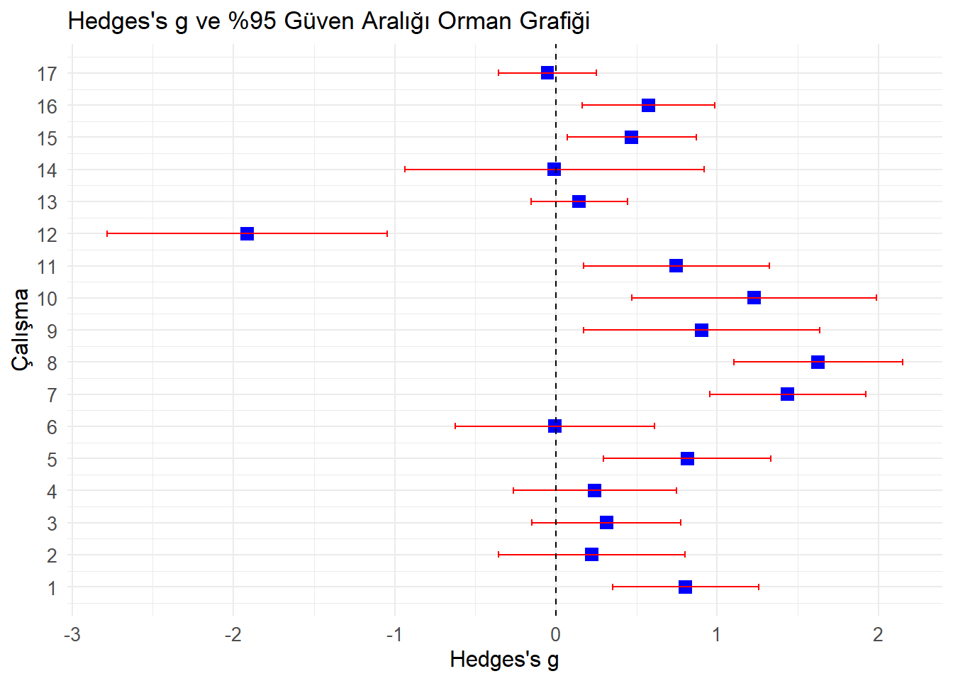
Heterojenlik testi
mean_exp <- data$mean_exp  # Deney grubunun aritmetik ortalaması
mean_control <- data$mean_control  # Kontrol grubunun aritmetik ortalaması
sd_exp <- data$sd_exp  # Deney grubunun standart sapması
sd_control <- data$sd_control  # Kontrol grubunun standart sapması
n_exp <- data$n_exp  # Deney grubunun örneklem büyüklüğü
n_control <- data$n_control  # Kontrol grubunun örneklem büyüklüğü
pooled_sd <- sqrt(((n_exp - 1) * sd_exp^2 + (n_control - 1) * sd_control^2) / (n_exp + n_control - 2))
pooled_sd
## [1] 17.819449 78.884420 22.492004 2.529160 2.545830 2.792380 13.073750
## [8] 14.021769 1.988328 1.542222 3.723882 10.499155 25.790450 43.294961
## [15] 11.353389 19.847399 10.073266# 2. Hedges's g hesaplama
g <- (mean_exp - mean_control) / pooled_sd * (1 - (3 / (4 * (n_exp + n_control - 2) - 1)))
g## [1] 0.804133004 0.221965382 0.312761326 0.241900890 0.814165649
## [6] -0.007016178 1.437180115 1.627394878 0.905283031 1.230235840
## [11] 0.747501202 -1.916011848 0.144756424 -0.008735008 0.469242550
## [16] 0.573185422 -0.052374997# 3. Hedges's g için Standart Hata (SE_g)
SE_g <- sqrt((n_exp + n_control) / (n_exp * n_control) + (g^2 / (2 * (n_exp + n_control)))) * (1 - (3 / (4 * (n_exp + n_control) - 9)))
SE_g## [1] 0.2305295 0.2949492 0.2356715 0.2579115 0.2651936 0.3146537 0.2469052
## [8] 0.2666053 0.3730337 0.3874314 0.2936914 0.4432254 0.1526744 0.4727295
## [15] 0.2042260 0.2094871 0.1543107## [1] 0.05314383 0.08699506 0.05554104 0.06651832 0.07032764 0.09900697
## [7] 0.06096218 0.07107838 0.13915413 0.15010312 0.08625462 0.19644879
## [13] 0.02330948 0.22347321 0.04170828 0.04388486 0.02381179# 5. Güven Aralığı (95% CI)
z_critical <- 1.96 # 95% güven aralığı için
lower_ci <- g - z_critical * SE_g
upper_ci <- g + z_critical * SE_g
lower_ci## [1] 0.35229528 -0.35613513 -0.14915477 -0.26360556 0.29438620 -0.62373750
## [7] 0.95324593 1.10484852 0.17413700 0.47087022 0.17186613 -2.78473372
## [13] -0.15448542 -0.93528488 0.06895951 0.16259063 -0.35482395## [1] 1.2559707 0.8000659 0.7746774 0.7474073 1.3339451 0.6097051
## [7] 1.9211143 2.1499412 1.6364291 1.9896015 1.3231363 -1.0472900
## [13] 0.4439983 0.9178149 0.8695256 0.9837802 0.2500740## [1] 3.48820075 0.75255451 1.32710725 0.93792224 3.07008034 -0.02229809
## [7] 5.82077712 6.10413590 2.42681307 3.17536398 2.54519301 -4.32288326
## [13] 0.94813810 -0.01847781 2.29766265 2.73613659 -0.33941263## [1] 4.862828e-04 4.517177e-01 1.844732e-01 3.482844e-01 2.140012e-03
## [6] 9.822102e-01 5.857464e-09 1.033583e-09 1.523210e-02 1.496487e-03
## [11] 1.092174e-02 1.540032e-05 3.430592e-01 9.852577e-01 2.158100e-02
## [16] 6.216522e-03 7.342989e-01##
## --- Sabit Model Sonuçları ---## Q İstatistiği: 94.3856## I^2: 83.04826## Tau Kare: 0##
## --- Rasgele Model Sonuçları ---## Q İstatistiği: 94.3856## I^2: 87.44238## Tau Kare: 0.4268754# Sabit model için Cochran's Q hesaplama
Q_fixed <- sum((fixed_model$yi - fixed_model$beta)^2 / fixed_model$vi)## Warning in fixed_model$yi - fixed_model$beta: Recycling array of length 1 in vector-array arithmetic is deprecated.
## Use c() or as.vector() instead.# Rasgele model için Cochran's Q hesaplama
Q_random <- sum((random_model$yi - random_model$beta)^2 / random_model$vi)## Warning in random_model$yi - random_model$beta: Recycling array of length 1 in vector-array arithmetic is deprecated.
## Use c() or as.vector() instead.## [1] 94.3856## [1] 94.52604results <- data.frame(
study = 1:nrow(data),
mean_exp = mean_exp,
mean_control = mean_control,
pooled_sd = pooled_sd,
g = g,
SE_g = SE_g,
var_g = var_g,
lower_ci = lower_ci,
upper_ci = upper_ci,
z_value = z_value,
p_value = p_value
)
# Sonuçları görüntüle
print(results)## study mean_exp mean_control pooled_sd g SE_g var_g
## 1 1 70.71 56.27 17.819449 0.804133004 0.2305295 0.05314383
## 2 2 59.40 41.66 78.884420 0.221965382 0.2949492 0.08699506
## 3 3 33.71 26.60 22.492004 0.312761326 0.2356715 0.05554104
## 4 4 3.69 3.07 2.529160 0.241900890 0.2579115 0.06651832
## 5 5 5.17 3.07 2.545830 0.814165649 0.2651936 0.07032764
## 6 6 6.04 6.06 2.792380 -0.007016178 0.3146537 0.09900697
## 7 7 94.58 75.61 13.073750 1.437180115 0.2469052 0.06096218
## 8 8 98.67 75.61 14.021769 1.627394878 0.2666053 0.07107838
## 9 9 7.45 5.60 1.988328 0.905283031 0.3730337 0.13915413
## 10 10 4.40 2.45 1.542222 1.230235840 0.3874314 0.15010312
## 11 11 19.12 16.29 3.723882 0.747501202 0.2936914 0.08625462
## 12 12 45.71 66.43 10.499155 -1.916011848 0.4432254 0.19644879
## 13 13 50.50 46.75 25.790450 0.144756424 0.1526744 0.02330948
## 14 14 52.88 53.28 43.294961 -0.008735008 0.4727295 0.22347321
## 15 15 73.43 68.06 11.353389 0.469242550 0.2042260 0.04170828
## 16 16 55.91 44.44 19.847399 0.573185422 0.2094871 0.04388486
## 17 17 20.94 21.47 10.073266 -0.052374997 0.1543107 0.02381179
## lower_ci upper_ci z_value p_value
## 1 0.35229528 1.2559707 3.48820075 4.862828e-04
## 2 -0.35613513 0.8000659 0.75255451 4.517177e-01
## 3 -0.14915477 0.7746774 1.32710725 1.844732e-01
## 4 -0.26360556 0.7474073 0.93792224 3.482844e-01
## 5 0.29438620 1.3339451 3.07008034 2.140012e-03
## 6 -0.62373750 0.6097051 -0.02229809 9.822102e-01
## 7 0.95324593 1.9211143 5.82077712 5.857464e-09
## 8 1.10484852 2.1499412 6.10413590 1.033583e-09
## 9 0.17413700 1.6364291 2.42681307 1.523210e-02
## 10 0.47087022 1.9896015 3.17536398 1.496487e-03
## 11 0.17186613 1.3231363 2.54519301 1.092174e-02
## 12 -2.78473372 -1.0472900 -4.32288326 1.540032e-05
## 13 -0.15448542 0.4439983 0.94813810 3.430592e-01
## 14 -0.93528488 0.9178149 -0.01847781 9.852577e-01
## 15 0.06895951 0.8695256 2.29766265 2.158100e-02
## 16 0.16259063 0.9837802 2.73613659 6.216522e-03
## 17 -0.35482395 0.2500740 -0.33941263 7.342989e-01Veriler heterojenlik testine göre Q(sd=16) değeri 94,3856 (p<0,05) olarak bulunmuştur. Elde edilen Q değerinin ki-kare tablo değerinin (sd=16, p<0,05) 26,33’ün üzerinde olması verilerin heterojen olduğunu göstermektedir. Hesaplanan I-kare değeri %83,04826’ tür. Bu değer yüksek düzeyde heterojenlik olduğunu göstermektedir.