4 Ortalama Farklar
4.1 Standartlaştırılmamış Ortalama Farkı
Formül 1. \[ \begin{align} D &= \bar{X}_{G_1} - \bar{X}_{G_2} \\ S.H. &= S_B \cdot \sqrt{\frac{1}{n_{G_1}} + \frac{1}{n_{G_2}}} \\ S_B &= \sqrt{\frac{(n_{G_1}-1)S_{G_1}^2 + (n_{G_2}-1)S_{G_2}^2}{(n_{G_1}-1) + (n_{G_2}-1)}} \\ w &= \frac{1}{(S.H.)^2} \end{align} \]
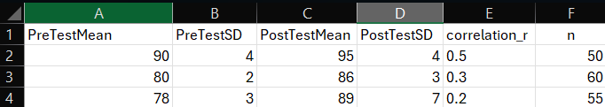
##   PreTestMean      PreTestSD    PostTestMean    PostTestSD    correlation_r
##  Min.   :78.00   Min.   :2.0   Min.   :86.0   Min.   :3.000   Min.   :0.2000
##  1st Qu.:79.00   1st Qu.:2.5   1st Qu.:87.5   1st Qu.:3.500   1st Qu.:0.2500
##  Median :80.00   Median :3.0   Median :89.0   Median :4.000   Median :0.3000
##  Mean   :82.67   Mean   :3.0   Mean   :90.0   Mean   :4.667   Mean   :0.3333
##  3rd Qu.:85.00   3rd Qu.:3.5   3rd Qu.:92.0   3rd Qu.:5.500   3rd Qu.:0.4000
##  Max.   :90.00   Max.   :4.0   Max.   :95.0   Max.   :7.000   Max.   :0.5000
##        n
##  Min.   :50.0
##  1st Qu.:52.5
##  Median :55.0
##  Mean   :55.0
##  3rd Qu.:57.5
##  Max.   :60.0
pre_test_mean <- data$PreTestMean
post_test_mean <- data$PostTestMean
pre_test_sd <- data$PreTestSD
post_test_sd <- data$PostTestSD
n <- data$n
correlation_r <- data$correlation_r
mean_diff <- post_test_mean - pre_test_mean # Ortalama farkı
mean_diff## [1] 5 6 11## [1] 4.000000 2.549510 5.385165## [1] 0.5656854 0.3894440 0.9184968## [1] 3.125000 6.593407 1.185345## [1] 5 6 11Formül 2.
\[ \begin{align} G &= \bar{X}_{T_1} - \bar{X}_{T_2} \\ S.H. &= \sqrt{\frac{2S_B^2(1-r)}{n}} \\ S_B &= \sqrt{\frac{S_{T_1}^2 + S_{T_2}^2}{2}} \\ w &= \frac{1}{(S.H.)^2} \end{align} \]
4.2 Standartlaştırılmış Ortalama Farkı
Formül 3.
Cohen d
\[ \begin{align} d &= \frac{\bar{X}_{G_1} - \bar{X}_{G_2}}{S_B} \\ S_B &= \sqrt{\frac{(n_{G_1}-1)S_{G_1}^2 + (n_{G_2}-1)S_{G_2}^2}{(n_{G_1}-1)+(n_{G_2}-1)}} \\ S.H. &= \sqrt{\frac{n_{G_1}+n_{G_2}}{n_{G_1}n_{G_2}} + \frac{d^2}{2(n_{G_1}+n_{G_2})}} \\ w &= \frac{1}{(S.H.)^2} \end{align} \]
Hedges g
\[ \begin{align} g &= \left(1 - \frac{3}{4sd - 9}\right) \cdot d \\ J &= 1 - \frac{3}{4sd - 9} \\ S.H.g &= J \cdot (S.H.d) \\ w &= \frac{1}{(S.H.g)^2} \end{align} \]
library(readxl)

# Excel dosyasını oku
data <- read_excel("s39.xlsx")

# Verilerdeki sütunları örnek olarak (değişkenler) belirleyelim
# Varsayalım ki 'pretest_mean', 'posttest_mean', 'pretest_sd', 'posttest_sd', 'n_pretest', 'n_posttest' gibi sütunlar var
pretest_means <- data$pretest_mean
posttest_means <- data$posttest_mean
pretest_sds <- data$pretest_sd
posttest_sds <- data$posttest_sd
n_pretest <- data$n_pretest
n_posttest <- data$n_posttest

# 1. Standartlaştırılmış Etki Büyüklüğü (Cohen's d)
cohen_d <- function(M_pre, M_post, SD_pre, SD_post, n_pre, n_post) {
  # Havuzlanmış standart sapmayı hesapla
  SD_pooled <- sqrt(((n_pre - 1) * SD_pre^2 + (n_post - 1) * SD_post^2) / (n_pre + n_post - 2))
  # Cohen's d hesapla
  d <- (M_pre- M_post) / SD_pooled
  return(d)
}

# 2. Cohen's d için Standart Hata (SE_d)
SE_d <- function(n_pre, n_post, d) {
  SE <- sqrt((n_pre + n_post) / (n_pre * n_post) + d^2 / (2 * (n_pre + n_post)))
  return(SE)
}

# 3. Hedge's g
hedges_g <- function(d, n_pre, n_post) {
  g <- d * (1 - (3 / (4 * (n_pre + n_post) - 9)))
  return(g)
}

# 4. Hedge's g için Standart Hata (SE_g)
SE_g <- function(SE_d, n_pre, n_post) {
  SE_g <- SE_d * (1 - (3 / (4 * (n_pre + n_post) - 9)))
  return(SE_g)
}

# 5. Ağırlık (W)
weight <- function(SE_d) {
  w <- 1 / (SE_d^2)
  return(w)
}

# Tüm makaleler için hesaplamaları yap
results <- data.frame(
  study = 1:nrow(data),
  d = numeric(nrow(data)),
  SE_d = numeric(nrow(data)),
  g = numeric(nrow(data)),
  SE_g = numeric(nrow(data)),
  w_d = numeric(nrow(data)),
  w_g = numeric(nrow(data))
)

for(i in 1:nrow(data)) {
  # Cohen's d hesapla
  d_val <- cohen_d(pretest_means[i], posttest_means[i], pretest_sds[i], posttest_sds[i], n_pretest[i], n_posttest[i])
  # Cohen's d için Standart Hata hesapla
  SE_d_val <- SE_d(n_pretest[i], n_posttest[i], d_val)
  # Hedge's g hesapla
  g_val <- hedges_g(d_val, n_pretest[i], n_posttest[i])
  # Hedge's g için Standart Hata hesapla
  SE_g_val <- SE_g(SE_d_val, n_pretest[i], n_posttest[i])
  # Ağırlık hesapla
  w_d_val <- weight(SE_d_val)
  w_g_val <- weight(SE_g_val)

  # Sonuçları sakla
  results[i, ] <- c(i, d_val, SE_d_val, g_val, SE_g_val, w_d_val, w_g_val)
}

# Sonuçları görüntüle
print(results)
## study d SE_d g SE_g w_d w_g
## 1 1 1.264911 0.4000000 1.230724 0.3891892 6.25000 6.602045
## 2 2 -2.666667 0.2748737 -2.646206 0.2727647 13.23529 13.440755
## 3 3 2.000000 0.1224745 1.996229 0.1222435 66.66667 66.918794Önceki bölümlerde tek grup ön test-son test karşılaştırmasını ve iki grubun son test ortalamalarının karşılaştırılmasını içeren durumlara yer verilmiştir. Öntest-sontest kontrol gruplu deneysel desen çalışmalarında Cohen d ve Hedges g indeksleri hesaplanabilmektedir.

Formül 4.
\[ \begin{align} d &= \frac{(\bar{X}_{G_{1SON}} - \bar{X}_{G_{1ÖN}}) - (\bar{X}_{G_{2SON}} - \bar{X}_{G_{2ÖN}})}{S_B} \\ S_B &= \sqrt{\frac{(n_{G_1}-1)S_{G_{1SON}}^2 + (n_{G_2}-1)S_{G_{2SON}}^2}{(n_{G_1}-1) + (n_{G_2}-1)}} \\ S.H. &= \sqrt{\frac{n_{G_1} + n_{G_2}}{n_{G_1} n_{G_2}} + \frac{d^2}{2(n_{G_1} + n_{G_2})}} \\ w &= \frac{1}{(S.H.)^2} \end{align} \]
library(readxl)
# Excel dosyasını oku
data <- read_excel("s45.xlsx")
# Veri setinizi kontrol et
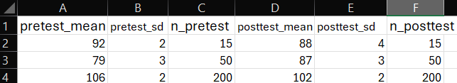
head(data)## # A tibble: 1 × 10
## exp_pre_mean exp_post_mean control_pre_mean control_post_mean exp_pre_sd
## <dbl> <dbl> <dbl> <dbl> <dbl>
## 1 80 90 80 84 2
## # ℹ 5 more variables: exp_post_sd <dbl>, control_pre_sd <dbl>,
## # control_post_sd <dbl>, n_exp <dbl>, n_control <dbl># Verilerdeki sütunları örnek olarak (değişkenler) belirleyelim
exp_pre_mean <- data$exp_pre_mean # Deneysel grup öntest aritmetik ortalama
exp_post_mean <- data$exp_post_mean # Deneysel grup sontest aritmetik ortalama
control_pre_mean <- data$control_pre_mean # Kontrol grup öntest aritmetik ortalama
control_post_mean <- data$control_post_mean # Kontrol grup sontest aritmetik ortalama
exp_pre_sd <- data$exp_pre_sd # Deneysel grup öntest standart sapma
exp_post_sd <- data$exp_post_sd # Deneysel grup sontest standart sapma
control_pre_sd <- data$control_pre_sd # Kontrol grup öntest standart sapma
control_post_sd <- data$control_post_sd # Kontrol grup sontest standart sapma
n_exp <- data$n_exp # Deney grubu için örneklem büyüklüğü
n_control <- data$n_control # Kontrol grubu için örneklem büyüklüğü
# 1. Deneysel ve Kontrol Grubu için Cohen's d hesapla
cohen_d <- function(M_exp_pre, M_exp_post, M_control_pre, M_control_post, SD_exp_pre, SD_exp_post, SD_control_pre, SD_control_post, n_exp, n_control) {
# Havuzlanmış standart sapmayı hesapla
SD_pooled <- sqrt(((n_exp - 1) * (SD_exp_post^2) +(n_control - 1) * (SD_control_post^2)) / (n_exp + n_control - 2)) # Toplam örneklem büyüklüğü - 2
# Cohen's d hesapla: (deney post-pre) - (kontrol post-pre) / SD_pooled
d <- ((M_exp_post - M_exp_pre) - (M_control_post - M_control_pre)) / SD_pooled
return(d)
}
# 2. Standart hata (SE) hesapla
standard_error <- function(n_exp, n_control, d) {
SE <- sqrt((1 / n_exp) + (1 / n_control)+ (d^2/(2* (n_exp+ n_control))))
return(SE)
}
# 3. Ağırlık (W) hesapla: W = 1 / SE^2
weight <- function(SE) {
w <- 1 / SE^2
return(w)
}
# 4. Deneysel ve Kontrol Grubu için hesaplamaları yap
results <- data.frame(
study = 1:nrow(data),
d = numeric(nrow(data)),
w = numeric(nrow(data))
)
for(i in 1:nrow(data)) {
# Cohen's d hesapla
d_val <- cohen_d(data$exp_pre_mean[i], data$exp_post_mean[i], data$control_pre_mean[i], data$control_post_mean[i],
data$exp_pre_sd[i], data$exp_post_sd[i], data$control_pre_sd[i], data$control_post_sd[i],
data$n_exp[i], data$n_control[i])
# Havuzlanmış standart sapmayı hesapla
SD_pooled <- sqrt(((data$n_exp[i] - 1) * data$exp_pre_sd[i]^2 + (data$n_exp[i] - 1) * data$exp_post_sd[i]^2 +
(data$n_control[i] - 1) * data$control_pre_sd[i]^2 + (data$n_control[i] - 1) * data$control_post_sd[i]^2) /
(data$n_exp[i] + data$n_control[i] - 2))
# Standart hata hesapla
SE_val <- standard_error(data$n_exp[i], data$n_control[i], d_val)
# Ağırlık (W) hesapla
w_val <- weight(SE_val)
# Sonuçları sakla
results[i, ] <- c(i, d_val, w_val, SE_val)
}## Warning in matrix(value, n, p): data length [4] is not a sub-multiple or
## multiple of the number of columns [3]## study d w
## 1 1 2 33.333334.3 Korelasyona Dayalı Etki Büyüklüğü
Formül 5.
Korelasyona dayalı etki büyüklüğü
\[ \begin{align} r_{xy} &= \frac{\sigma_{xy}^2}{\sigma_x \sigma_y} \\ V_r &= \frac{(1-r^2)^2}{n-1} \end{align} \]
Fisher’s z
\[ \begin{align} z &= 0.5 \cdot \ln\left(\frac{1+r}{1-r}\right) \\ r &= \frac{e^{2z} - 1}{e^{2z} + 1} \end{align} \]
library(readxl)
# Excel dosyasını oku
data <- read_excel("s47.xlsx")
# Veri setini kontrol et
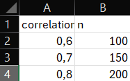
head(data)## # A tibble: 3 × 2
## correlation n
## <dbl> <dbl>
## 1 0.6 100
## 2 0.7 150
## 3 0.8 200# Verilerdeki korelasyon ve örneklem büyüklüğünü belirleyelim
r_values <- data$correlation # Korelasyon katsayıları
n_values <- data$n # Örneklem büyüklükleri
# 1. Fisher Z Dönüşümü (Korelasyonu Fisher Z'ye dönüştür)
fisher_z <- function(r) {
Z <- 0.5 * log((1 + r) / (1 - r))
return(Z)
}
# Fisher Z değerlerini hesapla
z_values <- sapply(r_values, fisher_z)
# 2. Standart hata (SE) hesaplama: SE_Z = 1 / sqrt(n - 3)
standard_error <- function(n) {
SE_Z <- 1 / sqrt(n - 3)
return(SE_Z)
}
# Standart hataları hesapla
se_values <- sapply(n_values, standard_error)
# 3. Ağırlıkları hesapla: W = 1 / SE_Z^2
weight <- function(SE_Z) {
W <- 1 / SE_Z^2
return(W)
}
# Ağırlıkları hesapla
weights <- sapply(se_values, weight)
# 4. Ağırlıklı Fisher Z hesaplama: Weighted Z = sum(W_i * Z_i) / sum(W_i)
weighted_z <- sum(weights * z_values) / sum(weights)
# 5. Ağırlıklı etki büyüklüğünü hesaplamak için Weighted Z'yi korelasyona dönüştür
r_weighted <- (exp(2 * weighted_z) - 1) / (exp(2 * weighted_z) + 1)
# Sonuçları yazdır
cat("Ağırlıklı Fisher Z değeri:", weighted_z, "\n")## Ağırlıklı Fisher Z değeri: 0.9323244## Ağırlıklı Korelasyon katsayısı (r): 0.7316758# Çalışma bazında sonuçları da görmek isterseniz:
results <- data.frame(
study = 1:nrow(data),
r = r_values,
z = z_values,
se = se_values,
weight = weights
)
# Sonuçları görüntüle
print(results)
## study r z se weight
## 1 1 0.6 0.6931472 0.10153462 97
## 2 2 0.7 0.8673005 0.08247861 147
## 3 3 0.8 1.0986123 0.07124705 197[Bu kitapta ikili veriye dayalı etki büyüklükleri bulunan kod verilmeyecektir.]