Chapter 9 Digression II: Survival analysis with R
One of the main advantages in using R is the abundance of maintained packages for a wide variety of statistical applications. An example of a commonly used statistical concept is survival analysis, also known as time-to-event analysis. Survival analysis is used to find the time until a specified event occurs - in most cases, this event is an outcome or an endpoint for a study. This outcome could be death of a patient or a disease re-occurrence (often used in clinical studies to study the relationship between patient survival and patient striations) or something mundane such as customer churning or a failure of a mechanical system. In R, such analysis can be handled trivially using syntax already familiar to us.
There are two functions critical to survival analysis: the survival function \(S(t)\) and the hazard function \(h(t)\) - both a function of time \(t\). The survival function describes the probability of surviving beyond time \(t\) without the event occurring. It describes the proportion of the sample which has not experienced the event up until \(t\). The hazard function describes the rate at which events occur at time \(t\), given that the sample has survived up until that time. Thus, a higher value of this rate denotes higher risk.
The Kaplan-Meier estimator is used to estimate the survival function \(S(t)\) given censored data. In this case, a data point is said to be censored if the sample (i.e., individual) does not experience the event during the study period. The Kaplan-Meier method is non-parametric, which means it does not make any assumptions about the distribution of the survival times. It also does not quantify the effect size (i.e., difference in risk between sample groups) but instead outputs the probability of survival at given time points.
\(\hat{S}(t)=\prod_{i:t_{i}\le t} (1-\frac{d_{i}}{n_{i}})\)
Here, \(\hat{S}(t)\) describes the probability of survival at \(t\), \(t\) is the time of interest, \(t_{i}\) is the times of event occurrences, \(d_{i}\) is the number of observed events, and \(n_{i}\) is the number of individuals at risk before \(t_{i}\). The product is evaluated over all event times \(t_{i}\) less than equal to the time point of interest \(t\). For each \(t_{i}\) then, \((1-\frac{d_{i}}{n_{i}})\) denotes the probability of surviving beyond \(t_{i}\).
Often, we frame our hypothesis to test whether there is a difference between two groups of individuals with respect to their survival probability. For example, we might be interested in whether, given patients enrolled in chemotherapy, men and women have different survival outcomes. Two survival functions can be subject to the log-rank test to compare the distributions:
\(\chi^{2}=\sum_{i}^{n}\frac{(O_{i}-E_{i})^{2}}{E_{i}}\)
Above, \(O_{i}\) is the number of observed events in group \(i\), while \(E_{i}\) is the number of expected events in \(i\). \(n\) is the number of groups being compared. The \(E_{i}\) term here can be calculated based on the Kaplan-Meier probabilities and the total number of observed events across the groups. The obtained log-rank test statistic is compared against the \(\chi^{2}\) distribution for statistical inference.
In R, the workhorse of survival analysis is the aptly named package survival and survminer.
library(tidyverse)
library(survival)
library(survminer)

df <- survival::ovarian %>% as_tibble()
df %>% glimpse()
## Rows: 26
## Columns: 6
## $ futime <dbl> 59, 115, 156, 421, 431, 448, 464, 475, 477, 563, 6…
## $ fustat <dbl> 1, 1, 1, 0, 1, 0, 1, 1, 0, 1, 1, 0, 0, 0, 0, 0, 0,…
## $ age <dbl> 72.3315, 74.4932, 66.4658, 53.3644, 50.3397, 56.43…
## $ resid.ds <dbl> 2, 2, 2, 2, 2, 1, 2, 2, 2, 1, 1, 1, 2, 2, 1, 1, 2,…
## $ rx <dbl> 1, 1, 1, 2, 1, 1, 2, 2, 1, 2, 1, 2, 2, 2, 1, 1, 1,…
## $ ecog.ps <dbl> 1, 1, 2, 1, 1, 2, 2, 2, 1, 2, 2, 1, 2, 1, 1, 2, 2,…I loaded the ovarian cancer dataset from the survival package. Here, we can striate the patients into two groups based on the rx column, which describes two different treatment regimen. The censor status as a binary variable is located in the fustat column, where 0 indicates censored, and 1 indicates death.
The Kaplan-Meier estimator is fit using survfit() on a survival object created by Surv(). Here, standard formula notation applies as we saw before.
## Call: survfit(formula = Surv(futime, fustat) ~ rx, data = df)
##
##       n events median 0.95LCL 0.95UCL
## rx=1 13      7    638     268      NA
## rx=2 13 5 NA 475 NA## # A tibble: 26 × 9
## time n.risk n.event n.censor estimate std.error conf.high
## <dbl> <dbl> <dbl> <dbl> <dbl> <dbl> <dbl>
## 1 59 13 1 0 0.923 0.0801 1
## 2 115 12 1 0 0.846 0.118 1
## 3 156 11 1 0 0.769 0.152 1
## 4 268 10 1 0 0.692 0.185 0.995
## 5 329 9 1 0 0.615 0.219 0.946
## 6 431 8 1 0 0.538 0.257 0.891
## 7 448 7 0 1 0.538 0.257 0.891
## 8 477 6 0 1 0.538 0.257 0.891
## 9 638 5 1 0 0.431 0.340 0.840
## 10 803 4 0 1 0.431 0.340 0.840
## # ℹ 16 more rows
## # ℹ 2 more variables: conf.low <dbl>, strata <chr>The survival plots are then drawn:
ggsurvplot(s, ggtheme = theme_survminer(),
           risk.table = 'abs_pct', pval = TRUE,
           risk.table.col = 'strata',
           palette = c("#a6f5c5", "#9d95bc"),
           surv.median.line = 'hv')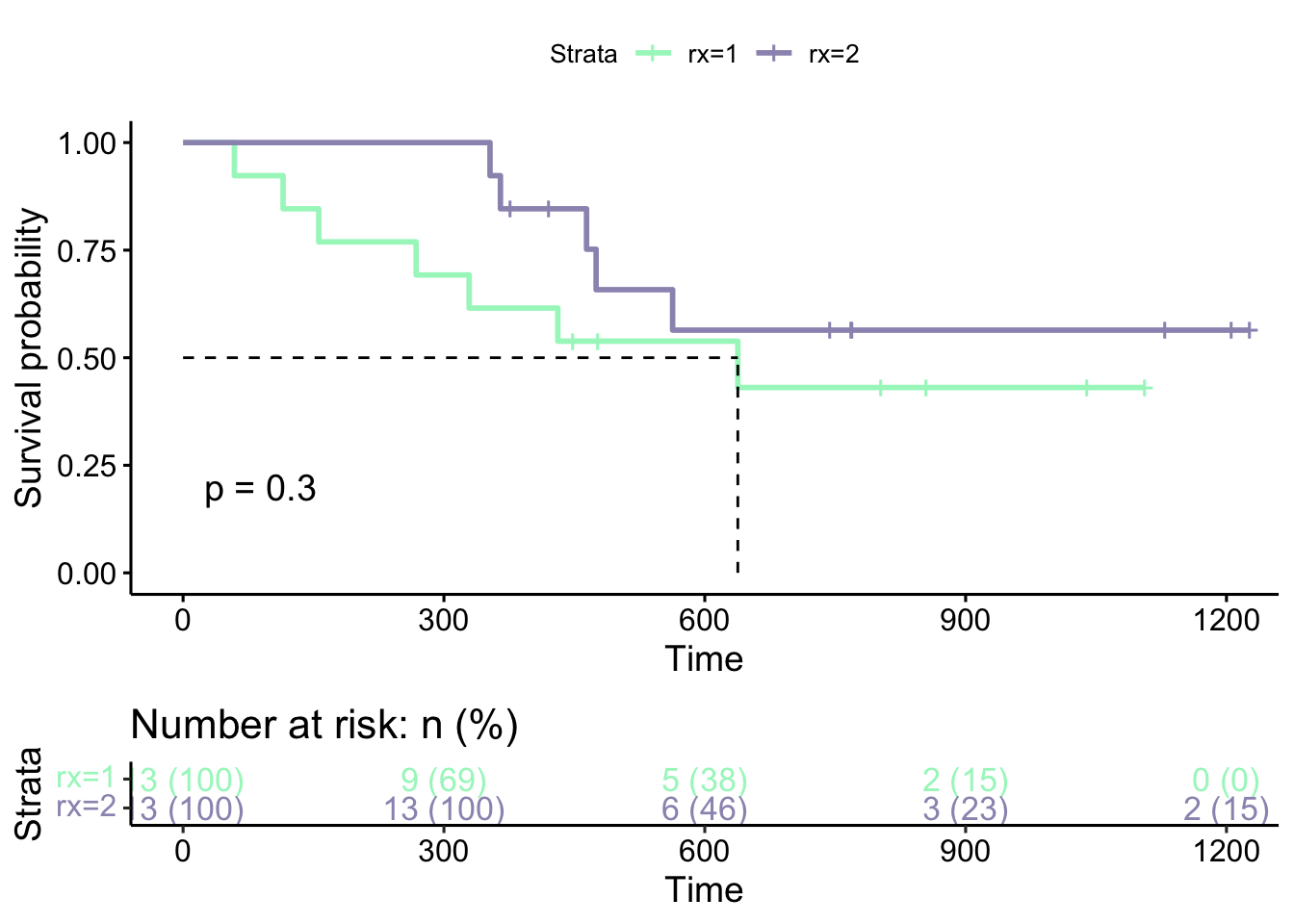
Here, the p-value (\(p=0.3\)) indicated on the figure is the p-value obtained from the log-rank test comparing the two groups. We can also extract this value by:
##   variable      pval   method pval.txt
## 1       rx 0.3025911 Log-rank  p = 0.3
The log-rank test and its associated values (such as the expected number of events) can formally be run using survdiff() as well:
## Call:
## survdiff(formula = Surv(futime, fustat) ~ rx, data = df)
##
##       N Observed Expected (O-E)^2/E (O-E)^2/V
## rx=1 13        7     5.23     0.596      1.06
## rx=2 13        5     6.77     0.461      1.06
##
##  Chisq= 1.1  on 1 degrees of freedom, p= 0.3
In order to quantify the difference in risk between the two groups, we use the hazard function.
\(h_{i}(t)=h_{0}(t)e^{\sum_{i}^{n}\beta x}\)
Here, \(h_{i}(t)\) denotes the hazard function for group \(i\), which is a function of time \(t\). It is then the exponential of the coefficient \(\beta\) obtained from model fitting which describes the effect size of the hazard function. The ratio between two hazard functions (i.e., between individuals or groups) then describes the relative difference in risk.
Therefore, it is evident that unlike the Kaplan-Meier estimator, hazard models output a list of coefficients for each covariate along with their p-values. This means that we are able to identify the magnitude and the direction of the association between each predictor variable and the hazard of experiencing the event.
Formally, the hazards regression model is fit in R using coxph() (stands for Cox proportional hazards model):
## Call:
## coxph(formula = Surv(futime, fustat) ~ rx, data = df, ties = "exact")
##
##   n= 26, number of events= 12
##
##       coef exp(coef) se(coef)      z Pr(>|z|)
## rx -0.5964    0.5508   0.5870 -1.016     0.31
##
##    exp(coef) exp(-coef) lower .95 upper .95
## rx    0.5508      1.816    0.1743      1.74
##
## Concordance= 0.608  (se = 0.07 )
## Likelihood ratio test= 1.05  on 1 df,   p=0.3
## Wald test            = 1.03  on 1 df,   p=0.3
## Score (logrank) test = 1.06  on 1 df,   p=0.3
Firstly, look at the last portion of the summary() output: the log-rank test is included in the model output as a test for overall difference in the groups. The p-value here should equal to the p-value we obtained previously for the log-rank test:
##      test        df    pvalue
## 1.0627399 1.0000000 0.3025911
Going back to the summary() output, the coef given equals the regression model coefficient \(\beta\). Here, since there are two groups, the first group (i.e., rx=1) is used as the reference. Here, the coef value of -0.5964 suggests that the rx=2 group have lower risk than the other, though obviously the result is not statistically significant. The effect size, or the hazard ratio then, is the exponential of this value, which is also given in the summary() output as 0.5508. This result suggests that the second group havs less risk of event than the other by a factor of 0.5508, or roughly 45%, at p-value of 0.31 (i.e., not significant).
The advantage of the hazard regression model is the ability to fit multiple predictors. This allows us to account for correlation between the predictor variables and identify potential associations.
The log-rank test returns a p-value of 3.14e-04, suggesting a difference between the groups.
##         test           df       pvalue
## 1.870381e+01 3.000000e+00 3.147869e-04
The summary() output on the multivariate model shows that there could be an association between patients’ age and hazard risk (\(\alpha < .05\)):
## Call:
## coxph(formula = Surv(futime, fustat) ~ rx + age + ecog.ps, data = df,
## ties = "exact")
##
## n= 26, number of events= 12
##
## coef exp(coef) se(coef) z Pr(>|z|)
## rx -0.8146 0.4428 0.6342 -1.285 0.1990
## age 0.1470 1.1583 0.0463 3.175 0.0015 **
## ecog.ps 0.1032 1.1087 0.6064 0.170 0.8649
## ---
## Signif. codes: 0 '***' 0.001 '**' 0.01 '*' 0.05 '.' 0.1 ' ' 1
##
## exp(coef) exp(-coef) lower .95 upper .95
## rx 0.4428 2.2582 0.1278 1.535
## age 1.1583 0.8633 1.0579 1.268
## ecog.ps 1.1087 0.9020 0.3378 3.639
##
## Concordance= 0.798 (se = 0.078 )
## Likelihood ratio test= 15.92 on 3 df, p=0.001
## Wald test = 13.32 on 3 df, p=0.004
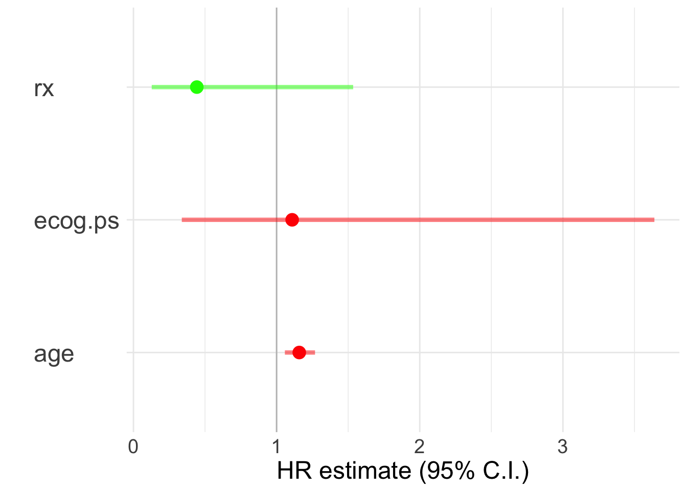
## Score (logrank) test = 18.7 on 3 df, p=3e-04A useful visualization to depict the respective hazard ratios is a linerange plot. For that we first need to do a bit of dplyr operations to obtain the confidence intervals and the hazard ratios.
c <- tidy(cox2)
c <- c %>% mutate(upper = estimate+1.96*std.error,
                  lower = estimate-1.96*std.error)
r <- c('estimate', 'upper', 'lower')
c <- c %>% mutate(across(all_of(r), exp))

ggplot(c, aes(x = estimate, y = term,
               color = estimate>1)) +
  geom_vline(xintercept = 1, color = 'gray') +
  geom_linerange(aes(xmin = lower, xmax = upper),
                 linewidth = 1.5, alpha = .5) +
  geom_point(size = 4) + theme_minimal() +
  scale_color_manual(values = c('green', 'red'),
                     guide = 'none') +
  theme(axis.text.y = element_text(hjust = 0, size = 18),
        text = element_text(size = 18)) +
  ylab('') + xlab('HR estimate (95% C.I.)')