Chapter 8 Digression I: Gradient descent with R
Previous two chapters covered two main facets of supervised models: classification and regression. Though it may seem trivial, one of the most important aspects of machine learning is the model training process. When training a model, one must consider both domain knowledge (which may aid in feature engineering) as well as model complexity. Related to these ideas is the concept of parameter space - therein which we can formally define the process of model training as searching for a combination of model parameters that minimizes a cost function. Now, this isn’t a ML book so there is no need to do a deep-dive here at all; however, the preceding definition can boil down to a simple task of minimizing error - a concept that extends to the simplest of models such as a simple linear model.
In brief, model training is an iterative process where we evaluate a prediction \(y(x_{i})\) over a training set, evaluate a loss (i.e., deviation between \(y(x_{i})\) and \(y\) - the ground truth), then tweak the model (i.e., model parameters) to minimize the loss.
In simple linear regression, this loss term is actually squared to account for deviations in either direction. This is called the square loss. Summing the square loss over the number of samples then, we get the mean squared error or MSE.
\(MSE=J(\theta_{1},\theta_{0})=\frac{1}{N}\sum_{i=1}^{N}(y(x_{i})-y_{i})^{2}\)
Here, \(\theta\) is the model’s parameter; since this is a simple linear regression (i.e., the familiar \(y=mx+b\)), \(\theta_{1}\) describes the slope and \(\theta_{0}\) the intercept (i.e., the bias term). Note that the MSE is a continuous function; it is differentiable everywhere and has just one global minimum. This makes gradient descent trivial, as we will see below.
In gradient descent, we will find a value of \(\theta\) that minimizes the MSE. This means that we will look for the derivative (in this case, it’s actually partial deriviatves since we have two terms - the slope and the intercept) of the cost function and tweak the model parameters in the opposite direction (so that we are going down the slope). This will ensure that we will (eventually) converge to a minimum value.
Keep in mind - here, we are looking for the local gradient descent with respect to \(\theta\). This means that the problem gets more challenging with complex cost functions with multiple local minima. This sounds annoying, but will not affect us in our example with the MSE.
Annoyingly, we have to do some math before we get implement gradient descent for our example. However, finding the partial derivatives for the MSE function is not too difficult:
For \(j = 0,1\):
\(\frac{\partial}{\partial \theta_{j}}J(\theta_{1},\theta_{0})=\frac{\partial}{\partial \theta_{j}}[\frac{1}{N}\sum_{i=1}^{N}(y(x_{i})-y_{i})^{2}]\)
\(\frac{\partial}{\partial \theta_{j}}J(\theta_{1},\theta_{0})=\frac{1}{N}\frac{\partial}{\partial \theta_{j}}\sum_{i=1}^{N}(y(x_{i})-y_{i})^{2}\)
After taking the constant \(\frac{1}{N}\) outside of the partial derivative, the RHS can be solved using the chain rule:
\(\frac{\partial}{\partial \theta_{j}}J(\theta_{1},\theta_{0})=\frac{1}{N}\sum_{i=1}^{N}2(y(x_{i})-y_{i})*\frac{\partial}{\partial \theta_{j}}(y(x_{i})-y_{i})\)
\(\frac{\partial}{\partial \theta_{j}}J(\theta_{1},\theta_{0})=\frac{1}{N}\sum_{i=1}^{N}2(y(x_{i})-y_{i})*(\frac{\partial}{\partial \theta_{j}}y(x_{i})\frac{\partial}{\partial \theta_{j}}y_{i})\)
The \(\frac{\partial}{\partial \theta_{j}}y_{i}\) term evaluates to zero since \(y_{i}\) is just a constant. Then:
\(\frac{\partial}{\partial \theta_{j}}J(\theta_{1},\theta_{0})=\frac{2}{N}\sum_{i=1}^{N}(y(x_{i})-y_{i})*\frac{\partial}{\partial \theta_{j}}y(x_{i})\)
The above equation describes a sum of residuals and a partial derivative term. The partial derivative term must be solved with respect to both the slope and the intercept. Firstly, for the intercept:
\(\frac{\partial}{\partial \theta_{0}}y(x_{i})=\frac{\partial}{\partial \theta_{0}}\theta_{i}x_{i}+\theta_{0}\)
\(\frac{\partial}{\partial \theta_{0}}y(x_{i})=\frac{\partial}{\partial \theta_{0}}\theta_{i}x_{i}+\frac{\partial}{\partial \theta_{0}}\theta_{0}\)
On the RHS, first term is a constant and second term evaluates to 1.
\(\frac{\partial}{\partial \theta_{0}}y(x_{i})=1\)
Solving the partial derivative for the slope then:
\(\frac{\partial}{\partial \theta_{1}}y(x_{i})=\frac{\partial}{\partial \theta_{0}}\theta_{i}x_{i}+\frac{\partial}{\partial \theta_{0}}\theta_{0}\)
On the RHS, first term evaluates to \(x_{i}\) and second term is a constant. So:
\(\frac{\partial}{\partial \theta_{1}}y(x_{i})=x_{i}\)
Finally, we can substitute the respective partial derivatives in the equation from before:
\(\frac{\partial}{\partial \theta_{0}}J(\theta_{1},\theta_{0})=\frac{2}{N}\sum_{i=1}^{N}y(x_{i})-y_{i}\)
\(\frac{\partial}{\partial \theta_{1}}J(\theta_{1},\theta_{0})=\frac{2}{N}\sum_{i=1}^{N}y(x_{i})-y_{i}*x_{i}\)
In words, the derivative with respect to the intercept term \(\theta_{0}\) is just the sum of residuals multipled by a constant. The deriative with respect to the slope \(\theta{1}\) is the same, but with an extra \(x_{i}\) term. For gradient descent, now that we’ve found the partial derivatives, we need to multiply these partial derivatives by a small factor (this factor is also called the learning rate) to find new values for the slope and the intercept.
Finally, let’s visualize this in R using the equation we’ve derived:
Here we’ve initialized the parameter values using random values (i.e., random initialization). We’ve also generated simulated data which we will fit a linear model on.
y <- theta_1*x + theta_0 + rnorm(n_obs, 0, 3)
data <- tibble(x = x, y = y)
ggplot(data, aes(x = x, y = y)) +
  geom_point(size = 2) + theme_bw() +
  labs(title = 'Simulated Data')
Now we fit a linear model using lm(), as seen previously:
##
## Call:
## lm(formula = y ~ x, data = data)
##
## Residuals:
##     Min      1Q  Median      3Q     Max
## -8.2671 -2.0105  0.0313  1.8922  8.2113
##
## Coefficients:
##             Estimate Std. Error t value Pr(>|t|)
## (Intercept)   4.9986     0.1357   36.84   <2e-16 ***
## x             1.8381     0.1395   13.18   <2e-16 ***
## ---
## Signif. codes:  0 '***' 0.001 '**' 0.01 '*' 0.05 '.' 0.1 ' ' 1
##
## Residual standard error: 3.032 on 498 degrees of freedom
## Multiple R-squared:  0.2585, Adjusted R-squared:  0.257
## F-statistic: 173.6 on 1 and 498 DF,  p-value: < 2.2e-16
Let’s print out the model parameters:
## (Intercept)           x
##    4.998597    1.838081
Now we define a function to calculate the MSE:
cost_function <- function(theta_0, theta_1, x, y){
  pred <- theta_1*x + theta_0
  res_sq <- (y - pred)^2
  res_ss <- sum(res_sq)
  return(mean(res_ss))
}

cost_function(theta_0 = ols$coefficients[1][[1]],
         theta_1 = ols$coefficients[2][[1]],
         x = data$x, y = data$y)
## [1] 4577.087## [1] 4577.087Now, for the gradient descent: in the function below, delta_theta_0 and delta_theta_1 corresponds to the two derived equations earlier from the partial derivatives. We also define the learning rate alpha and the number of iterations iter.
gradient_desc <- function(theta_0, theta_1, x, y){
  N = length(x)
  pred <- theta_1*x + theta_0
  res <- y - pred
  delta_theta_0 <- (2/N)*sum(res)
  delta_theta_1 <- (2/N)*sum(res*x)
  return(c(delta_theta_0, delta_theta_1))
}

alpha <- 0.1
iter <- 100
Using the function gradient_desc(), we define a function to tweak the model parameters by the obtained partial derivatives scaled by alpha:
minimize_function <- function(theta_0, theta_1, x, y, alpha){
  gd <- gradient_desc(theta_0, theta_1, x, y)
  d_theta_0 <- gd[1] * alpha
  d_theta_1 <- gd[2] * alpha
  new_theta_0 <- theta_0 + d_theta_0
  new_theta_1 <- theta_1 + d_theta_1
  return(c(new_theta_0, new_theta_1))
}
For the random initialization, we will use 0 and 0 and then progressively iterate through the gradient descent algorithm (iter number of times) and examine the parameter values at the end.
res <- list()
res[[1]] <- c(0, 0)

for (i in 2:iter){
  res[[i]] <- minimize_function(
    res[[i-1]][1], res[[i-1]][2], data$x, data$y, alpha
  )
}

res <- lapply(res, function(x) as.data.frame(t(x))) %>% bind_rows()
colnames(res) <- c('theta0', 'theta1')

loss <- res %>% as_tibble() %>% rowwise() %>%
  summarise(mse = cost_function(theta0, theta1, data$x, data$y))

res <- res %>% bind_cols(loss) %>%
  mutate(iteration = seq(1, 100)) %>% as_tibble()

res
## # A tibble: 100 × 4
## theta0 theta1 mse iteration
## <dbl> <dbl> <dbl> <int>
## 1 0 0 18985. 1
## 2 1.01 0.382 13725. 2
## 3 1.82 0.685 10385. 3
## 4 2.46 0.925 8265. 4
## 5 2.98 1.12 6918. 5
## 6 3.39 1.27 6064. 6
## 7 3.71 1.39 5521. 7
## 8 3.97 1.48 5176. 8
## 9 4.18 1.55 4958. 9
## 10 4.35 1.61 4819. 10
## # ℹ 90 more rowsFrom the tibble above, we can see that the parameter values (slope and intercept) approach what we’ve gotten earlier from the linear model (1.83 and 4.99, respectively). The MSE also decreases over iterations, which we can visualize:
ggplot(res, aes(x = iteration, y = mse)) +
  geom_point(size = 2) +
  theme_classic() + geom_line(aes(group = 1)) +
  labs(title = 'Gradient descent over 100 iterations')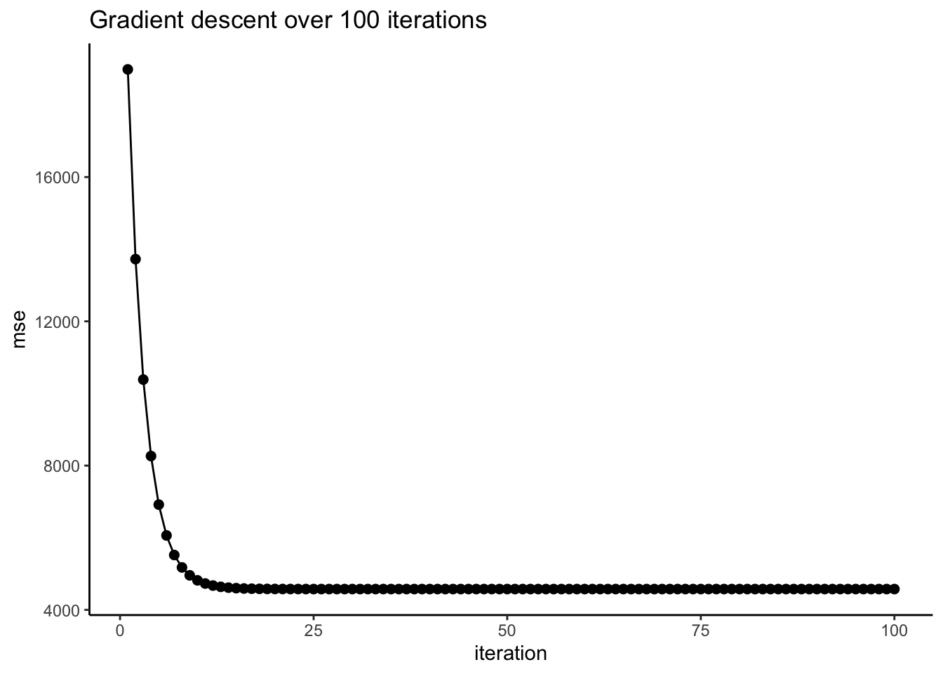
As a visual aid to see how gradient descent is working, we can visualize the regression line at each iteration over our synthetic data. Here, the blue line indicates the regression line at the first iteration, which has a slope and intercept of 0 (since we initialized them at 0). Over the 100 iterations, the regression line approaches the line of best fit we obtained earlier using lm(). The green line indicates the line at the 100th iteration.
ggplot(data, aes(x = x, y = y)) +
  geom_point(size = 2) +
  geom_abline(aes(intercept = theta0, slope = theta1),
              data = res, linewidth = 0.5, color = 'red') +
  theme_classic() +
  geom_abline(aes(intercept = theta0, slope = theta1),
              data = res %>% slice_head(),
              linewidth = 0.5, color = 'blue') +
  geom_abline(aes(intercept = theta0, slope = theta1),
              data = res %>% slice_tail(),
              linewidth = 0.5, color = 'green') +
  labs(title = 'Gradient descent over 100 iterations')