Chapter 3 S&P Predictions
3.1 Downloading S&P 500 daily Data
# S&P Daily Data

sp_data <- tq_get("^GSPC",
                 get = "stock.prices",
                 from = "1900-01-01",
                 to = "2022-10-01"
)


# dow_data <- tq_get("^DJI",
#                  get = "stock.prices",
#                  from = "1900-01-01",
#                  to = "2022-10-01"
# )

sp_data = sp_data %>% select(symbol, date,close)

sp_data
## # A tibble: 23,802 x 3
## symbol date close
## <chr> <date> <dbl>
## 1 ^GSPC 1927-12-30 17.7
## 2 ^GSPC 1928-01-03 17.8
## 3 ^GSPC 1928-01-04 17.7
## 4 ^GSPC 1928-01-05 17.5
## 5 ^GSPC 1928-01-06 17.7
## 6 ^GSPC 1928-01-09 17.5
## 7 ^GSPC 1928-01-10 17.4
## 8 ^GSPC 1928-01-11 17.4
## 9 ^GSPC 1928-01-12 17.5
## 10 ^GSPC 1928-01-13 17.6
## # ... with 23,792 more rowsNow, let’s add on some more columns that we know we’ll want to use in our analysis later on:
- \(PriceChange = Price_t - Price_{t-1}\)
- \(Return = \frac{(Price_t - Price_{t-1})}{Price_{t-1}}\)
sp_data = sp_data %>% mutate(price_change = close - lag(close),
                   ret = price_change/ lag(close),
                   lag_price = lag(close),
                   year = year(date),
                   month = month(date),
                   week = week(date),
                   day = day(date)
                   ) %>% drop_na()

sp_data
## # A tibble: 23,801 x 10
## symbol date close price_change ret lag_p~1 year month week day
## <chr> <date> <dbl> <dbl> <dbl> <dbl> <dbl> <dbl> <dbl> <int>
## 1 ^GSPC 1928-01-03 17.8 0.100 0.00566 17.7 1928 1 1 3
## 2 ^GSPC 1928-01-04 17.7 -0.0400 -0.00225 17.8 1928 1 1 4
## 3 ^GSPC 1928-01-05 17.5 -0.170 -0.00959 17.7 1928 1 1 5
## 4 ^GSPC 1928-01-06 17.7 0.110 0.00627 17.5 1928 1 1 6
## 5 ^GSPC 1928-01-09 17.5 -0.160 -0.00906 17.7 1928 1 2 9
## 6 ^GSPC 1928-01-10 17.4 -0.130 -0.00743 17.5 1928 1 2 10
## 7 ^GSPC 1928-01-11 17.4 -0.0200 -0.00115 17.4 1928 1 2 11
## 8 ^GSPC 1928-01-12 17.5 0.120 0.00692 17.4 1928 1 2 12
## 9 ^GSPC 1928-01-13 17.6 0.110 0.00630 17.5 1928 1 2 13
## 10 ^GSPC 1928-01-16 17.3 -0.290 -0.0165 17.6 1928 1 3 16
## # ... with 23,791 more rows, and abbreviated variable name 1: lag_price3.2 EDA
How about a little brief EDA, just to make sure we get a sense for what’s going on??
ggplot(sp_data,aes(date,close)) + geom_line()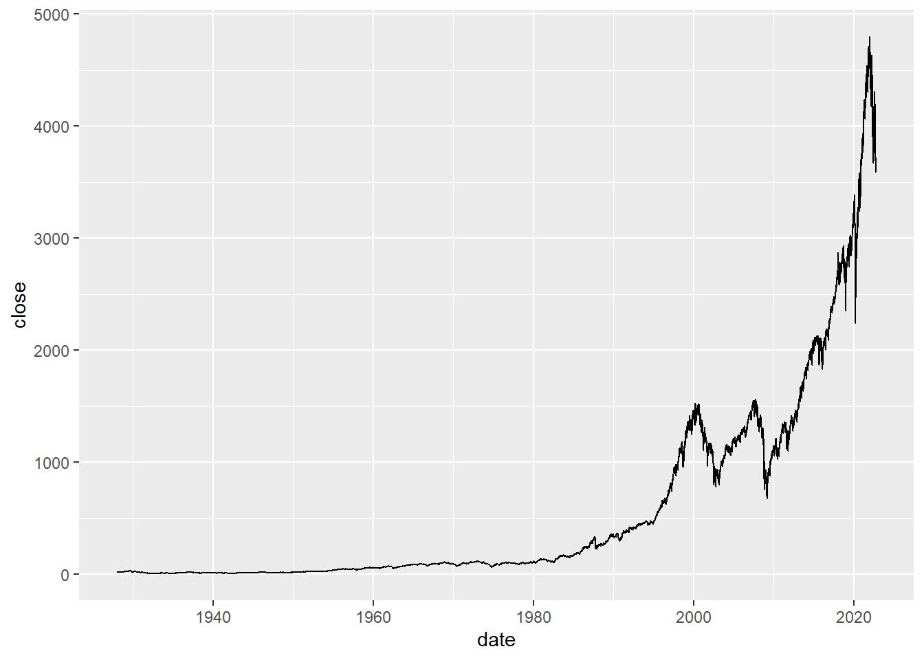
Well that is kind of hard to read. Maybe log transforming it will make it more interesting?
sp_data %>% mutate(log_price = log2(close)) %>%
  ggplot(aes(date,log_price)) + geom_line()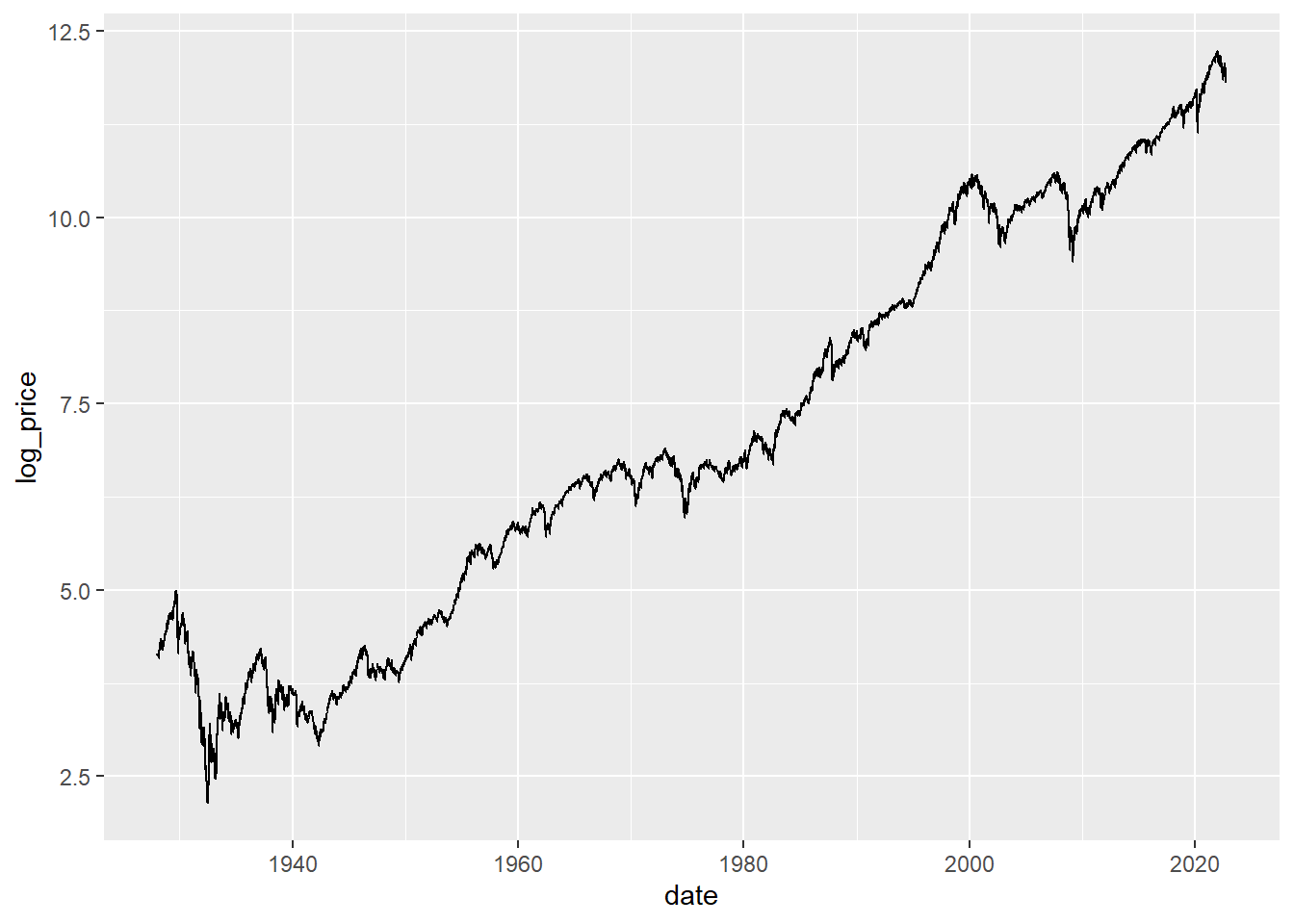
I suppose the takeaway from above analysis is that the S&P 500 does tend to go up over time. Not sure if that is really all that insightful.
But we can see below that the price change is clearly no where near constant overtime.
sp_data %>% ggplot(aes(date,price_change)) + geom_point()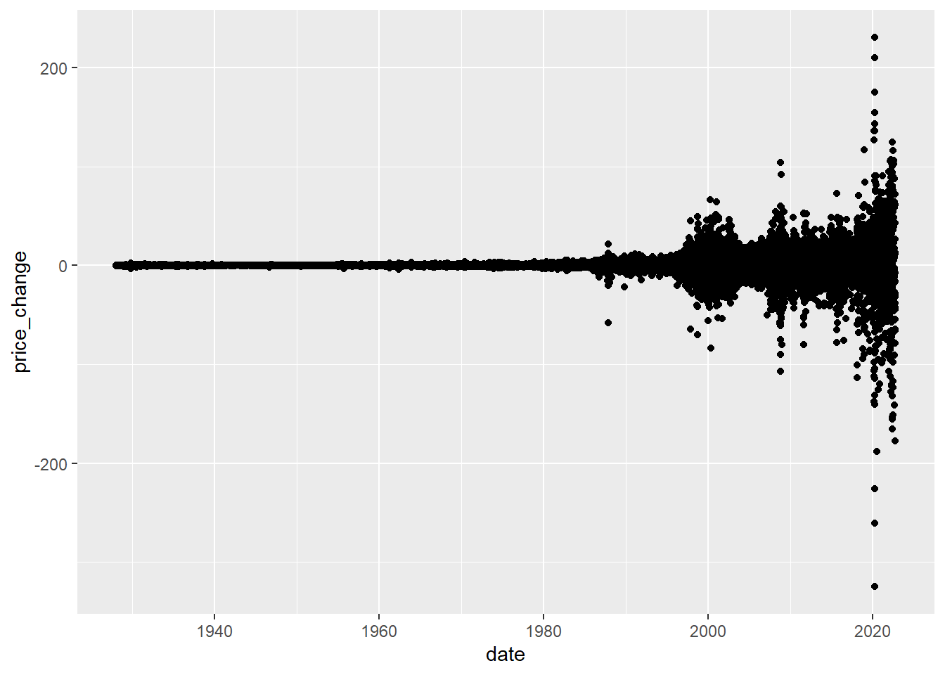
One of the takeaways I’d see from here is that there seem to be periods of high-volatility: big % changes are followed by big % changes.
sp_data %>% ggplot(aes(date,ret)) + geom_point()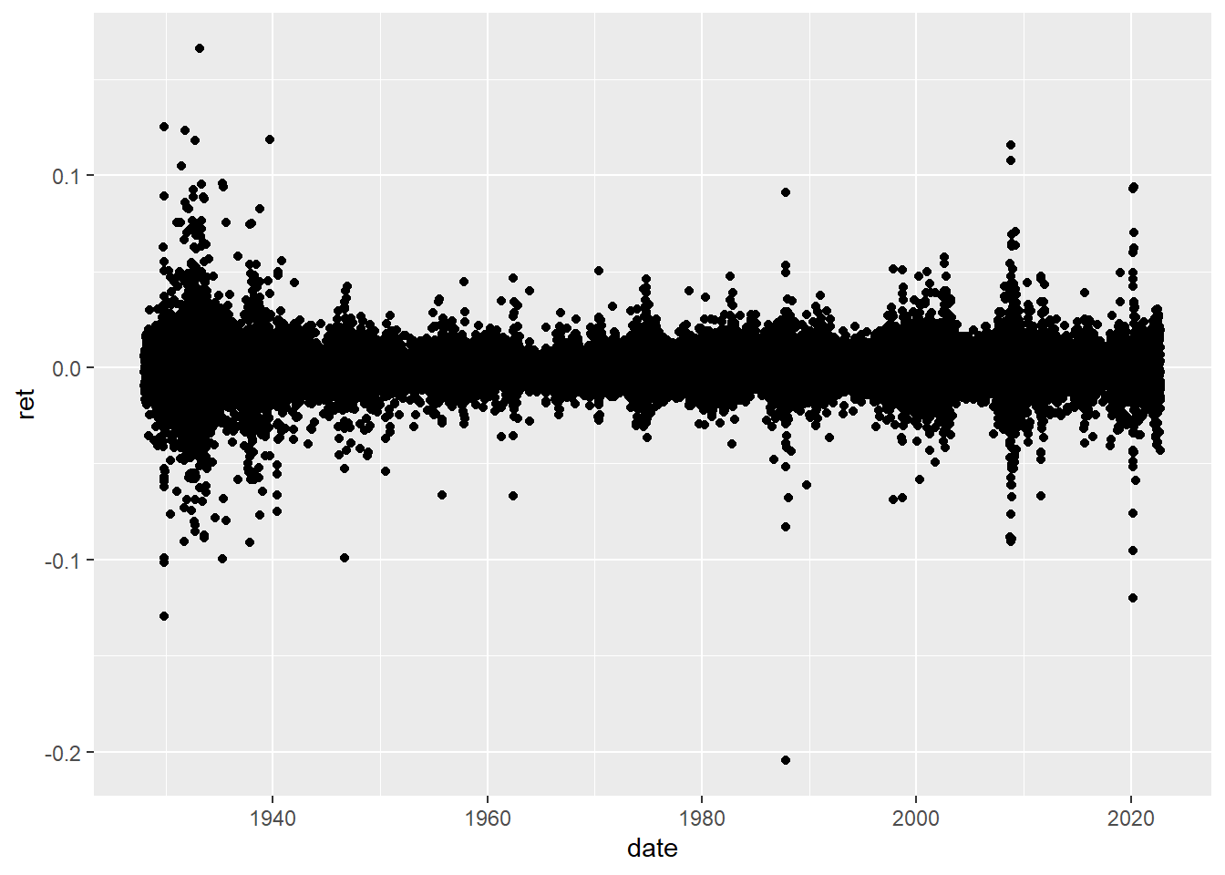
3.3 Modeling
EDA should give us some idea of the proper mathematical models to use to fit the data.
3.3.2 Linear Regression
mod = lm(close ~ lag_price,sp_data)
summary(mod)
##
## Call:
## lm(formula = close ~ lag_price, data = sp_data)
##
## Residuals:
## Min 1Q Median 3Q Max
## -325.35 -0.49 -0.05 0.46 229.96
##
## Coefficients:
## Estimate Std. Error t value Pr(>|t|)
## (Intercept) 6.978e-02 9.289e-02 0.751 0.453
## lag_price 1.000e+00 8.843e-05 11309.374 <2e-16 ***
## ---
## Signif. codes: 0 '***' 0.001 '**' 0.01 '*' 0.05 '.' 0.1 ' ' 1
##
## Residual standard error: 12.11 on 23799 degrees of freedom
## Multiple R-squared: 0.9998, Adjusted R-squared: 0.9998
## F-statistic: 1.279e+08 on 1 and 23799 DF, p-value: < 2.2e-16plot(sp_data$lag_price,mod$residuals)