MAT 4880 Mathematical Modeling II
Lecture Notes Experiment
2021-03-13
Chapter 1 Fitting a Logistic Model to Data
Example 1.1 We are given population data concerning the growth of a species of yeast in a closed vessel. Use the data given below and the solution \(u(t)\) to the logistic differential equation to find estimates of the parameters \(u_0\), \(r\) and \(K\).
\[u(t) = \frac{K}{1+e^{-rt} \left (\frac{K}{u_0}-1 \right )}\] where \(K\) is the carrying capacity of the population, \(r\) is the growth rate and \(u_0\) is the initial population size at time \(t=0\). For more details, please review the lectures where we covered all details related to the solution of the logistic equation.
We use a graphical approach for this problem to develop some intuition about fitting the logistic model parameters to given data.
- What is \(u_0\)?
- What is a good estimate for \(K\)? What do you predict as the maximum sustainable population (carrying capacity), based on this model?
- What is a good estimate for \(r\)? Adjust the value of \(r\) manually until the logistic solution fits the data well.
p (in millions) as a function of time t (in hours), is given by the data below:
t<-0:17 # time in hours
# population in millions
p<-c(9.6, 18.3, 29.0, 47.2, 71.1, 119.1, 174.6, 257.3, 350.7,
 441.0, 513.3, 559.7, 594.8, 629.4, 640.8, 651.1, 655.9, 659.6)
Hints:
- Start by creating a scatterplot of the data of yeast population against time.
- Find the horizontal asymptote to \(u(t)\) by finding \(\lim_{t\to\infty}u(t)\).
- Does the solution to the logistic equation level out? What is that level?
- Use the last observation above to make a good guess for the value of \(K\).
Problem Solution:
# load the required packages
library(mosaic)
library(mosaicCalc)
First, we plot the population size p against time t, using the data given above. We use the plotting function gf_point(), which is available when you load the mosaic package to visualize the data. Note that the plotting function takes a formula p ~ t, where p and t are the given data vectors, and it creates the scatterplot of p against t:
gf_point(p ~ t)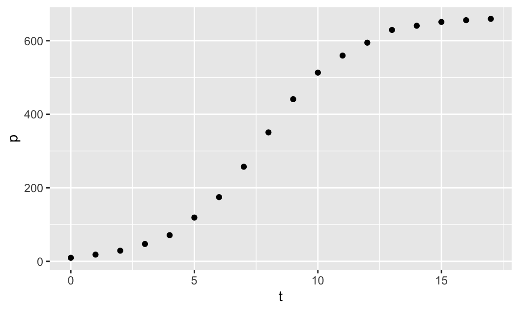
Next, we define the logistic solution as an R function u (the dependent variable) with argument t (the independent variable) using makeFun() from the mosaic package. Note that the R function u also depends on the parameters u0, r and K and it is created using the formula u(t) ~ t, which makes u a function of t:
u<-makeFun(K/(1+exp(-r*t)*(K/u0 - 1)) ~ t)The initial yeast population at time zero is p[1]=9.6, based on the data, so the parameter for the initial population is u0=9.6.
To find the horizontal asymptote, we need to find \(\lim_{t\to\infty}u(t)\). As \(t\to\infty\) the term \(e^{-rt}\) goes to 0:
\[\lim_{t\to\infty}u(t) = \lim_{t\to\infty}\frac{K}{1+0\cdot (K/u_0 -1)} = K\] Thus, the horizontal asymptote is \(u=K\) (on the \(tu\)-plane). The yeast data appear to converge to the horizontal level of around 670, so we can take this as a reasonable estimate for \(K=670\) to be the carrying capacity. We can plot the horizontal asymptote \(u=670\) along with the data to make sure that it fits the data well:
gf_point(p ~ t) %>%
  gf_hline(yintercept=670, col="red")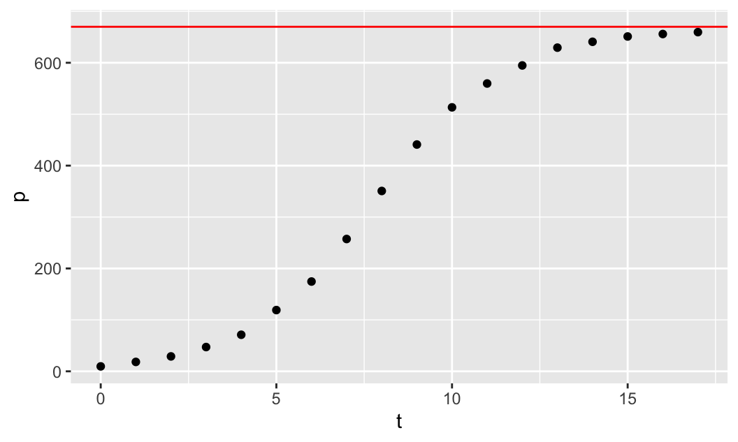
In the code above, after we create the scatterplot of the data using gf_point(p ~ t), we then use the pipe operator %>%, which implements a composition of functions, and it composes the first plotting function with the second plotting function gf_hline, which plots the horizontal line \(u=670\), for which we only need to specify the yintercept=670 (col="red" is optional).
Finally, to find a good estimate for \(r\), we can manually adjust the value of \(r\) until we get a good fit to the data. Note that we first create the scatter plot of the data as before, using gf_point(p ~ t), and then we use the pipe operator %>% to compose the two plotting functions. The second plotting function, composed with the first one, is the slice_plot() function from the mosaicCalc package. Note that slice_plot() takes the formula u(t,r=r, u0=u0, K=K) ~ t, where we give the parameters r, u0 and K specific numerical values and leave u to be a function of time t only. We then specify the domain over which to plot the graph of the function u(t) by giving a range for t, t=range(0,20) (col="blue" is optional).
u0=9.6 # initial population
K=670  # carrying capacity
r=0.54 # growth rate
gf_point(p ~ t) %>%
  slice_plot(u(t,r=r, u0=u0, K=K) ~ t, domain(t=range(0,20)),
             col="blue")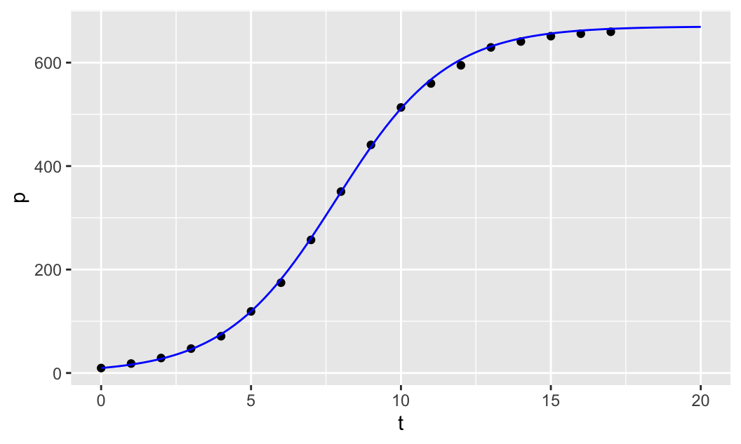
We then start to manually adjust the parameter r until the model fits the data well.
Manually adjusting the parameter \(r\) seems to produce a reasonable fit when \(r\approx 0.54\).