A Methodology
In this Section, we discuss the GraphR model and priors in Section A.1 and brief introduction to variational Bayes inference method with mean-field assumption in Section A.2 followed by detailed derivation of the update equations and evidence lower bound (ELBO) for our GraphR model in Section A.3 and Section A.4 respectively. In Section A.6, we provide a comprehensive overview of the GraphR and competing methods.
For notational purposes, we consider \(\mathbf{Y} = (Y_1,...,Y_p) \in \mathbb{R}^ {N \times p} \sim \mathcal{N}(\mu,\Omega^{-1}(\mathbf{X}))\), where the precision matrix \(\Omega(\mathbf{X}) = [\omega_{ij}(\mathbf{X})]_{p \times p}\) is a function of intrinsic factors \(\mathbf{X} = (X_1,...,X_q) \in \mathbb{R}^ {N \times q}\) and denote \(\boldsymbol{\theta}\) as the parameters of estimation. Here \(N\), \(p\), \(q\) denotes sample size, number of features and covariates respectively.
A.1 Model and priors
The GraphR model is expressed as follows: \[\begin{equation} \begin{split} & Y_i = \sum_{j \neq i}^p \gamma_{ij}(\mathbf{X}) \odot Y_j + \epsilon_i, \hspace{0.5cm} \epsilon_i \sim N(0,\frac{1}{\omega_{ii}}), \\ & \gamma_{ij}(X) = -\frac{\omega_{ij}(\mathbf{X})}{\omega_{ii}} = -\frac{1}{\omega_{ii}} \mathbf{X} \boldsymbol{\beta_{ij}} = -\frac{1}{\omega_{ii}} \left(\sum_{l=1}^q \beta_{ijl}X_l \right) \end{split} \tag{A.1} \end{equation}\] where \(\odot\) represents the element-wise multiplication between vectors.
Priors on the GraphR model are given below: \[\begin{align} \begin{split} & \beta_{ijl} = b_{ijl} s_{ijl}, \\ & b_{ijl} \mid \tau_{il} \sim N (0,\tau_{il}^{-1}), \\ & s_{ijl} \mid \pi_{ijl} \sim \text{Ber}(\pi_{ijl}), \\ & \tau_{il} \sim \text{Gamma}(a_\tau,b_\tau) \\ & \pi_{ijl} \sim \text{Beta}(a_\pi,b_\pi) \\ & \omega_{ii} \propto 1. \\ \end{split} \tag{A.2} \end{align}\]
Parameters of estimation are \(\boldsymbol{\theta} = \{ \boldsymbol{b,s,\omega,\pi,\tau}\}\).
A.2 Mean field variational Bayes
Varitional Bayes method aims to obtain the optimal approximation of true posterior distribution from a class of tractable distributions \(Q\), called variational family, by minimizing the Kullback-Leibler (KL) divergence between the approximate \(q_{\text{vb}}(\boldsymbol{\theta})\) and the true posterior distribution \(p(\boldsymbol{\theta|\mathbf{Y,X}})\) (Attias et al. 2000). A common choice of \(Q\), known as mean-field approximation, assumes that \(q_{\text{vb}}(\boldsymbol{\theta})\) can be expressed as \(\prod_{k=1}^K q^k_{\text{vb}}(\boldsymbol{\theta_k})\) for some partition of \(\boldsymbol{\theta}\). One can write \(q_{\text{vb}}(\boldsymbol{\theta})\) as
\[\begin{align}\label{eq:KL_div} & q_{\text{vb}}^{*}(\boldsymbol{\theta}) \in \text{arg} \underset{q_{\text{vb}}(\boldsymbol{\theta}) \in \mathbb{Q}}{\text{min}} \ KL(q_{\text{vb}}(\boldsymbol{\theta})\|p(\boldsymbol{\theta |Y,X})) \text{, where} \nonumber \\ & KL(q_{\text{vb}}(\boldsymbol{\theta})\|p(\boldsymbol{\theta|Y,X})) = \int q_{\text{vb}}(\boldsymbol{\theta}) \text{ log} \left (\frac{q_{\text{vb}}(\boldsymbol{\theta})}{p(\boldsymbol{\theta|Y,X})}\right)d\boldsymbol{\theta} \nonumber \\ & = - \int q_{\text{vb}}(\boldsymbol{\theta}) \text{ log} \left (\frac{p(\boldsymbol{\theta|Y,X})}{q_{\text{vb}}(\boldsymbol{\theta})}\right)d\boldsymbol{\theta} = - \int q_{\text{vb}}(\boldsymbol{\theta}) \text{ log} \left (\frac{p(\boldsymbol{\theta,Y,X})}{q_{\text{vb}}(\boldsymbol{\theta})}\right)d\boldsymbol{\theta} + \text{ log} \left[ p(\boldsymbol{Y,X}) \right]. \end{align}\]
We denote \(L[q_{\text{vb}}(\boldsymbol{\theta})] = \int q_{\text{vb}}(\boldsymbol{\theta}) \text{log} \left ( p(\boldsymbol{\theta,Y,X}) / q_{\text{vb}}(\boldsymbol{\theta}) \right)d\boldsymbol{\theta}\) which is the lower bound of the model log-likelihood, and write \(KL(q_{\text{vb}}(\boldsymbol{\theta})\|p(\boldsymbol{\theta|Y,X})) = -L[q_{\text{vb}}(\boldsymbol{\theta})] + \text{ log} \left[ p(\boldsymbol{Y,X}) \right]\). Minimizing KL-divergence is equivalent to maximizing \(L[q_{\text{vb}}(\boldsymbol{\theta})]\) since \(\text{ log} \left[ p(\boldsymbol{Y,X}) \right]\) doesn’t involve \(\boldsymbol{\theta}\). We can further show that \[\begin{align}\label{eq:lowerbound} L[q_{\text{vb}}(\boldsymbol{\theta})] &= \int q_{\text{vb}}(\boldsymbol{\theta}) \left[ \text{ log }p(\boldsymbol{\theta,Y,X}) - \text{ log } q_{\text{vb}}(\boldsymbol{\theta}) \right] d\boldsymbol{\theta} \nonumber \\ & = \int q^{k}_{\text{vb}}(\boldsymbol{\theta_k}) \int \left[ \left(\text{ log }p(\boldsymbol{\theta,Y,X}) - \text{ log }q_{\text{vb}}(\boldsymbol{\theta_k}) \right) \right] \prod_{i \neq k} q_{\text{vb}}(\boldsymbol{\theta_i}) d\boldsymbol{\theta_{-k}}d\boldsymbol{\theta_k} \nonumber \\ & \text{ } -\int \sum_{i \neq k} \text{ log }q_{\text{vb}}(\boldsymbol{\theta_i}) \prod_{i \neq k} q_{\text{vb}}(\boldsymbol{\theta_i}) \int q_{\text{vb}}(\boldsymbol{\theta_k}) d\boldsymbol{\theta_{-k}}d\boldsymbol{\theta_k} \nonumber \\ &= \int q^{k}_{\text{vb}}(\boldsymbol{\theta_k}) \left[\mathbb{E}_{-k} (\text{ log }p(\boldsymbol{\theta,Y,X})) - \text{ log } q_{\text{vb}}(\boldsymbol{\theta_k})\right] d\boldsymbol{\theta_k} - \text{const} \nonumber \\ &=-KL(q^{k}_{\text{vb}}(\boldsymbol{\theta_k}) \| \text{ exp } \left[ \mathbb{E}_{-k} (\text{ log }p(\boldsymbol{\theta,Y,X})) \right]). \end{align}\]
Therefore, we have \(q^{k}_{\text{vb}}(\boldsymbol{\theta_k}) \propto \text{ exp } \left[ \mathbb{E}_{-k} (\text{ log }p(\boldsymbol{\theta,Y,X})) \right]\).
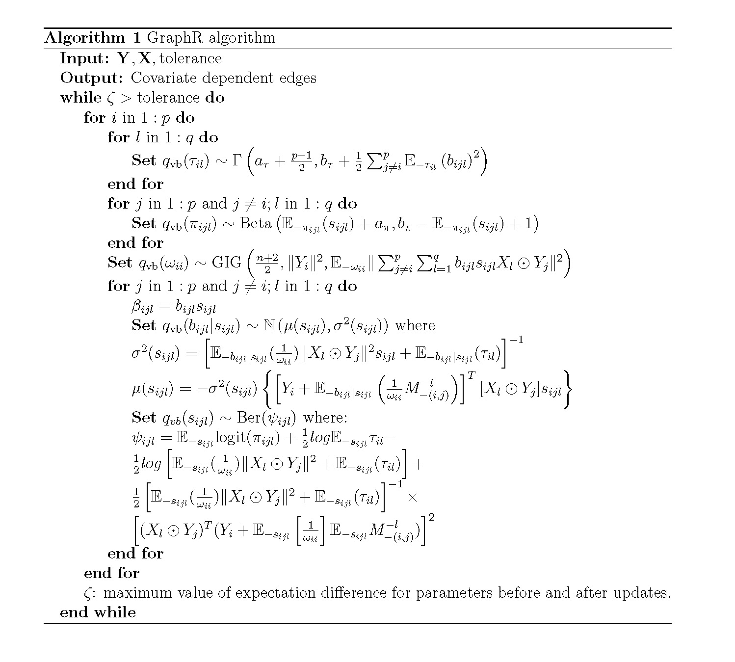
A.3 Update equations
The likelihood is expressed as \[\begin{align} p(\boldsymbol{\theta,Y,X}) &\propto \prod_{i=1}^p \left\{ \left| \frac{1}{\omega_{ii}}I_n \right|^{-\frac{1}{2}} \text{exp} \left[ -\frac{\omega_{ii}}{2} \left\| Y_i - \sum_{j \neq i} \gamma_{ij}(X) \odot Y_j \right \|^2 \right] \right\} \times \nonumber \\ & \prod_{i=1}^p \prod_{j \neq i}^p \prod_{l=1}^q \left\{\left(\frac{1}{\tau_{il}}\right)^{-\frac{1}{2}} \text{exp} \left[-\frac{\tau_{il}}{2}(b_{ijl})^2 \right] \left(\pi_{ijl}\right)^{s_{ijl}} \left(1-\pi_{ijl}\right)^{1-s_{ijl}} \right\} \times \nonumber \\ &\prod_{i=1}^p \prod_{l=1}^q \left\{ \left(\tau_{il} \right) ^ {a_\tau-1} \text{exp}\left[ -b_\tau \tau_{il} \right] \right\} \times \nonumber \\ &\prod_{i=1}^p \prod_{j \neq i}^p \prod_{l=1}^q\left\{ \left(\pi_{ijl}\right)^{a_\pi-1} \left(1-\pi_{ijl}\right)^{b_\pi-1} \right\} \end{align}\]
\[\begin{align} \text{log} p(\boldsymbol{\theta,Y,X}) = &\text{Const}+ \sum_{i=1}^p \left\{ \frac{n}{2} \text{log}(\omega_{ii}) - \frac{\omega_{ii}}{2} \left\| Y_i + \frac{1}{\omega_{ii}} \sum_{j \neq i}^p \sum_{l=1}^q b_{ijl} s_{ijl} X_l \odot Y_j \right \|^2 \right\} \nonumber \\ &+ \sum_{i=1}^p \sum_{l=1}^q \left\{ \left( \frac{p-1}{2} + a_\tau-1 \right) \text{log}(\tau_{il}) - \left( b_\tau + \frac{1}{2}\sum_{j \neq i}^p \left( b_{ijl} \right)^2 \right) \tau_{il} \right\} \nonumber \\ &+ \sum_{i=1}^p \sum_{j \neq i}^p \sum_{l=1}^q \left\{ \left( s_{ijl} + a_\pi -1 \right)\text{log}(\pi_{ijl}) + \left( b_\pi-s_{ijl} \right) \text{log}(1-\pi_{ijl}) \right\}. \end{align}\]
Due to the dependence between \(\boldsymbol{b}\) and \(\boldsymbol{s}\) (Titsias and Lázaro-Gredilla 2011), the mean-field assumption is considered as: \[q_{\text{vb}}(\boldsymbol{b,s,\omega,\pi,\tau}) = q_{\text{vb}}(\boldsymbol{b,s})q_{\text{vb}}(\boldsymbol{\omega})q_{\text{vb}}(\boldsymbol{\pi})q_{\text{vb}}(\boldsymbol{\tau}).\]
We can obtain the update equation for each parameter as \(q^{k}_{\text{vb}}(\boldsymbol{\theta_k}) \propto \text{ exp } \left[ \mathbb{E}_{-k} (\text{ log }p(\boldsymbol{\theta,Y,X})) \right]\).
a. Update of \(\tau_{il}\): \[\begin{align} \text{log} \ q_{\text{vb}}(\tau_{il}) &= \mathbb{E}_{-\tau_{il}} (l) \nonumber\\ &= C + \left[ \frac{p-1}{2}+a_\tau-1 \right] \text{log} \tau_{il} + \left[ b_\tau + \frac{1}{2}\sum_{j \neq i}^p \mathbb{E}_{-\tau_{il}} \left( b_{ijl} \right)^2 \right] \tau_{il}. \end{align}\]
\[q_{\text{vb}}(\tau_{il}) \sim \Gamma \left(a_\tau + \frac{p-1}{2}, b_\tau + \frac{1}{2}\sum_{j \neq i}^p \mathbb{E}_{-\tau_{il}}\left( b_{ijl} \right)^2 \right)\]
b. Update of \(\pi_{ijl}\):
\[\begin{align}
\text{log} \ q_{\text{vb}}(\pi_{ijl})
&= \mathbb{E}_{-\pi_{ijl}} (l) \nonumber \\
&= C+
\left[
\mathbb{E}_{-\pi_{ijl}}(s_{ijl})+a_\pi-1
\right] \text{log}(\pi_{ijl}) +
\left[
b_\pi - \mathbb{E}_{-\pi_{ijl}}(s_{ijl})
\right] \text{log}(1-\pi_{ijl}).
\end{align}\]
\[q_{\text{vb}}(\pi_{ijl}) \sim \text{Beta} \left(\mathbb{E}_{-\pi_{ijl}}(s_{ijl})+a_\pi, b_\pi - \mathbb{E}_{-\pi_{ijl}}(s_{ijl}) +1 \right)\]
c. Update \(\omega_{ii}\):
\[\begin{align}
\text{log} \ q_{\text{vb}}(\omega_{ii})
&= \mathbb{E}_{-\omega_{ii}}(l) \nonumber \\
&= C+
\frac{n}{2} \text{log}(\omega_{ii}) -\frac{\|Y_i\|^2}{2} \omega_{ii} - \frac{\mathbb{E}_{-\omega_{ii}}\|\sum_{j \neq i}^p \sum_{l=1}^q b_{ijl}s_{ijl}
X_l \odot Y_j\|^2}{2} \left( \frac{1}{\omega_{ii}} \right).
\end{align}\]
\[q_{\text{vb}}(\omega_{ii}) \sim \text{GIG} \left(\frac{n+2}{2},\|Y_i\|^2, \mathbb{E}_{-\omega_{ii}}\|\sum_{j \neq i}^p \sum_{l=1}^q b_{ijl}s_{ijl} X_l \odot Y_j\|^2 \right)\] Here GIG represents generalized inverse Gaussian distribution.
d. Update \(\beta_{ijl} = b_{ijl}s_{ijl}\):
\(\text{We Denote } M_{-(m,n)}^{-k} = \sum_{j \neq m }^p \sum_{l=1 }^q b_{mjl} s_{mjl} X_l \odot Y_j - b_{mnk} s_{mnk}X_k \odot Y_n\) and \[\begin{align} \text{log} \ q_{\text{vb}}(b_{ijl}|s_{ijl}) &= \mathbb{E}_{-b_{ijl}|s_{ijl}}(l) \nonumber \\ &= C-\frac{1}{2} \left[ \mathbb{E}_{-b_{ijl}|s_{ijl}}(\tau_{il}) + \mathbb{E}_{-b_{ijl}|s_{ijl}} \left( \frac{1}{\omega_{ii}} \right) s_{ijl} \|X_l \odot Y_j \|^2 \right] \left(b_{ijl} \right)^2 \nonumber \\ &-\left[Y_i+\mathbb{E}_{-b_{ijl}|s_{ijl}} \left( \frac{1}{\omega_{ii}} \right)\mathbb{E}_{-b_{ijl}|s_{ijl}}M_{-(i,j)}^{-l} \right]^T \left[X_l \odot Y_j \right] s_{ijl} b_{ijl}. \end{align}\]
\[q_{\text{vb}}(b_{ijl}|s_{ijl}) \sim \mathbb{N} \left(\mu(s_{ijl}),\sigma^2(s_{ijl})\right)\] \[\sigma^2(s_{ijl}) = \left[ \mathbb{E}_{-b_{ijl}|s_{ijl}}(\frac{1}{\omega_{ii}})\|X_l \odot Y_j\|^2 s_{ijl} + \mathbb{E}_{-b_{ijl}|s_{ijl}}(\tau_{il}) \right]^{-1}\]
\[\mu(s_{ijl}) = - \sigma^2(s_{ijl}) \left\{ \left[Y_i + \mathbb{E}_{-b_{ijl}|s_{ijl}} \left(\frac{1}{\omega_{ii}} M_{-(i,j)}^{-l} \right) \right]^T [X_l \odot Y_j] s_{ijl} \right\}\]
The mariginal density of \(q_{\text{vb}}(s_{ijl})\) is obtained by integrating the joint density of \(q_{\text{vb}}(b_{ijl},s_{ijl})\) as
\[\begin{align*}
\begin{split}
& q_{\text{vb}}(s_{ijl}) = \int \text{exp} \left\{ \text{log} \ q_{\text{vb}}(b_{ijl},s_{ijl}) \right\}db_{ijl} \\
& = \text{exp} \left\{
s_{ijl} \ \mathbb{E}_{-s_{ijl}} \text{logit}(\pi_{ijl})\right\}\ \int \mathbb{N}_{b_{ijl}}
\left(\mu(s_{ijl}),\sigma^2(s_{ijl})\right) \sigma(s_{ijl})
\text{exp } \left(
\frac{\mu^2(s_{ijl})}{2\sigma^2(s_{ijl})}\right) db_{ijl} \\
& = \sigma(s_{ijl})
\text{exp} \left\{
s_{ijl} \ \mathbb{E}_{-s_{ijl}} \text{logit}(\pi_{ijl}) + \left(
\frac{\mu^2(s_{ijl})}{2\sigma^2(s_{ijl})}\right)
\right\}. \\
& \text{log} [q_{\text{vb}}(s_{ijl})] =
C + \text{log}(\sigma(s_{ijl})) +
s_{ijl} \ \mathbb{E}_{-s_{ijl}} \text{logit}(\pi_{ijl}) +
\frac{\mu^2(s_{ijl})}{2\sigma^2(s_{ijl})} \\
& \text{log} [q_{\text{vb}}(s_{ijl}=0)] = C - \frac{1}{2} \text{log} \mathbb{E}_{-s_{ijl}}\tau_{ijl} \\
& \text{log} [q_{\text{vb}}(s_{ijl}=1)] = C +\mathbb{E}_{-s_{ijl}} \text{logit}(\pi_{ijl})
- \frac{1}{2} \text{log} \left[\mathbb{E}_{-s_{ijl}}(\frac{1}{\omega_{ii}})\|X_l \odot Y_j\|^2 + \mathbb{E}_{-s_{ijl}}(\tau_{il}) \right] \\
& + \frac{1}{2}\left[\mathbb{E}_{-s_{ijl}}(\frac{1}{\omega_{ii}})\|X_l \odot Y_j\|^2 + \mathbb{E}_{-s_{ijl}}(\tau_{il}) \right]^{-1}\left[(X_l \odot Y_j)^T (Y_i + \mathbb{E}_{-s_{ijl}} \left(\frac{1}{\omega_{ii}}\right) \mathbb{E}_{-s_{ijl}} M_{-(i,j)}^{-l}) \right]^2
\end{split}
\end{align*}\]
\[\begin{equation*} \begin{split} & s_{ijl} \sim \text{Ber}(\psi_{ijl}) \\ & \text{log} \ q_{\text{vb}}(s_{ijl}) = C + s_{ijl}\text{logit}(\psi_{ijl}) \\ & \psi_{ijl} = \mathbb{E}_{-s_{ijl}} \text{logit}(\pi_{ijl}) - \frac{1}{2}log\left[ \mathbb{E}_{-s_{ijl}}(\frac{1}{\omega_{ii}})\|X_l \odot Y_j\|^2 + \mathbb{E}_{-s_{ijl}}(\tau_{il}) \right] + \frac{1}{2}log \mathbb{E}_{-s_{ijl}} \tau_{il} \\ &+ \frac{1}{2}\left[ \mathbb{E}_{-s_{ijl}}(\frac{1}{\omega_{ii}})\|X_l \odot Y_j\|^2 + \mathbb{E}_{-s_{ijl}}(\tau_{il}) \right]^{-1}\left[ (X_l \odot Y_j)^T (Y_i + \mathbb{E}_{-s_{ijl}}\left[\frac{1}{\omega_{ii}}\right] \mathbb{E}_{-s_{ijl}} M_{-(i,j)}^{-l}) \right]^2 \\ \end{split} \end{equation*}\]
A.4 Evidence lower bound (ELBO)
As shown previously, the evidence lower bound is defined as:
\[\begin{equation*} \begin{split} L[q_{\text{vb}}(\boldsymbol{\theta})] &= \int q_{\text{vb}}(\boldsymbol{\theta}) \text{log} \left ( p(\boldsymbol{\theta,Y,X}) / q_{\text{vb}}(\boldsymbol{\theta}) \right)d\boldsymbol{\theta} \\ & = \mathbb{E}_{q_{\text{vb}}(\boldsymbol{\theta})} \text{ log}(p(\boldsymbol{\theta,Y,X})) - \mathbb{E}_{q_{\text{vb}}(\boldsymbol{\theta})} [q_{\text{vb}}(\boldsymbol{\theta})] \\ & = \mathbb{E}_{q_{\text{vb}}(\boldsymbol{\theta})} \text{ log}(p(\boldsymbol{\theta,Y,X})) - \sum_{i=1}^p \mathbb{E}_{q_{\text{vb}}(\boldsymbol{\theta})} [q_{\text{vb}}(\omega_{ii})] - \sum_{i=1}^p \sum_{l=1}^q \mathbb{E}_{q_{\text{vb}}(\boldsymbol{\theta})} [q_{\text{vb}}(\tau_{il})] \\ & - \sum_{i=1}^p \sum_{j \neq i}^p \sum_{l=1}^q \left\{ \mathbb{E}_{q_{\text{vb}}(\boldsymbol{\theta})} [q_{\text{vb}}(b_{ijl},s_{ijl})] + \mathbb{E}_{q_{\text{vb}}(\boldsymbol{\theta})} [q_{\text{vb}}(\pi_{ijl})] \right\}. \end{split} \end{equation*}\] Notably, \(-\mathbb{E}_{q_{\text{vb}}(\boldsymbol{\theta})} [q_{\text{vb}}(\omega_{ii})] , -\mathbb{E}_{q_{\text{vb}}(\boldsymbol{\theta})} [q_{\text{vb}}(\tau_{il})], -\mathbb{E}_{q_{\text{vb}}(\boldsymbol{\theta})} [q_{\text{vb}}(b_{ijl},s_{ijl})], -\mathbb{E}_{q_{\text{vb}}(\boldsymbol{\theta})} [q_{\text{vb}}(\pi_{ijl})]\) are entropies of GIG, Gamma, Normal, Bernoulli and Beta distributions, which have a close form. We denote entropy as \(H(\cdot)\) and all the expectations below are taken w.r.t \(q_{\text{vb}}(\boldsymbol{\theta})\).
a. Derivation of \(\mathbb{E} \text{ log}(p(\boldsymbol{\theta,Y,X}))\):
\[\begin{align*} \begin{split} \mathbb{E} \text{ log}(p(\boldsymbol{\theta,Y,X})) = & \sum_{i=1}^p \biggl \{ -\frac{n + (p-1)q}{2} \text{log} 2\pi + q \left[ a_\tau \text{log}b_\tau - \text{log} \Gamma(a_\tau) \right] \\ & + (p-1)q \left[ \text{log} \Gamma(a_\pi + b_\pi) -\text{log} \Gamma(a_\pi b_\pi) \right] \\ & + \frac{n}{2} \mathbb{E}(\text{log}\omega_{ii}) -\frac{\|Y_i\|^2}{2} \mathbb{E}\omega_{ii} -\mathbb{E}(\omega_{ii}^{-1}) \mathbb{E} \left\| \sum_{j \neq i}^p \sum_{l=1}^q \beta_{ijl} Z_l \odot Y_j \right \|^2 \\ & - Y_i^T \left(\sum_{j \neq i}^p \sum_{l=1}^q \mathbb{E} \beta_{ijl} Z_l \odot Y_j \right) \\ & + \sum_{l=1}^q \left[ \left( \frac{p-1}{2} + a_\tau-1 \right) \mathbb{E} \left(\text{log} \tau_{il} \right) - \left( b_\tau + \frac{\sum_{j \neq i}^p \mathbb{E}b_{ijl}^2}{2} \right) \mathbb{E} \tau_{il} \right] \\ & + \sum_{j \neq i}^p \sum_{l=1}^q \left[ \left( \mathbb{E}s_{ijl}+a_\pi - 1 \right) \mathbb{E} (\text{log} \pi_{ijl}) + (b_\pi - \mathbb{E}s_{ijl}) \right] \mathbb{E} \left(\text{log} (1-\pi_{ijl}) \right) \biggl \} \end{split} \end{align*}\]
b. Derivation of \(H(\tau_{il})\) \[\begin{align*} \begin{split} H(\tau_{il}) = & - \left[a_\tau+\frac{p-1}{2}\right] \text{log}\left[b_\tau + \frac{1}{2}\sum_{j \neq i} ^p\mathbb{E}b_{ijl}^2\right] + \text{log } \Gamma(a_\tau+\frac{p-1}{2}) \\ & - \left[a_\tau+\frac{p-1}{2} -1 \right] \mathbb{E}(\text{log }\tau_{il}) + \left[b_\tau + \frac{1}{2}\sum_{j \neq i} ^p\mathbb{E}b_{ijl}^2\right] \mathbb{E}\tau_{il} \end{split} \end{align*}\]
c. Derivation of \(H(\pi_{ijl})\) \[\begin{align*} \begin{split} H(\pi_{ijl}) = & - \text{log }\Gamma(a_\pi+b_\pi+1) + \text{log } \Gamma(\mathbb{E}s_{ijl} + a_\pi) + \text{log } \Gamma(b_\pi + 1 - \mathbb{E}s_{ijl}) \\ & - (\mathbb{E}s_{ijl} + a_\pi -1) \mathbb{E} \text{log } \pi_{ijl} - (b_\pi - \mathbb{E}s_{ijl}) \mathbb{E} \text{log } (1-\pi_{ijl}) \end{split} \end{align*}\]
d. Derivation of \(H(\omega_{ii})\)
Denote \(a_{\omega_{ii}} = \|Y_i\|^2\) and \(b_{\omega_{ii}} = \mathbb{E}\|\sum_{j \neq i}^p \sum_{l=1}^q \beta_{ijl} Z_l \odot Y_j\|^2\)
\[H(\omega_{ii}) = -\frac{n+2}{4} \text{log}\frac{a_{\omega_{ii}}}{b_{\omega_{ii}}} + \text{log}(2K_{(n+2)/2}\sqrt{a_{\omega_{ii}} b_{\omega_{ii}}}) -\frac{n}{2}\mathbb{E}(\text{log}\omega_{ii})+ \frac{a_{\omega_{ii}}}{2}\mathbb{E}\omega_{ii} + \frac{b_{\omega_{ii}}}{2}\mathbb{E}\omega_{ii}^{-1}\]
e. Derivation of \(H(b_{ijl}, s_{ijl})\) \[H(b_{ijl}, s_{ijl}) = H(b_{ijl}|s_{ijl}) + H(s_{ijl})\] where \[H(b_{ijl}|s_{ijl}) = \frac{1}{2} \text{log} \left[2\pi\sigma^2(s_{ijl})\right] + \frac{1}{2}\]
\[H(s_{ijl}) = -\psi_{ijl} \text{ log}(\psi_{ijl}) - (1-\psi_{ijl}) \text{ log}(1-\psi_{ijl})\]
Combining all the previous entropy derivations, we have the following expression of evidence lower bound (ELBO) as $ \[\begin{align*} \begin{split} L[q_{\text{vb}}(\boldsymbol{\theta})] = & -\frac{np + p(p-1)q}{2} \text{log} 2\pi \\ & + p q \left[ a_\tau \text{log}b_\tau - \text{log} \Gamma(a_\tau) + \text{log} \Gamma(a_\tau + \frac{p-1}{2}) \right] \\ & + p(p-1)q \left[ \text{log} \Gamma(a_\pi + b_\pi) -\text{log} \Gamma(a_\pi b_\pi) -\text{log} \Gamma(a_\pi+b_\pi+1) \right] \\ & - \sum_{i=1}^p \left\{ Y_i^T \left( \sum_{j \neq i}^p \sum_{l=1}^q \mathbb{E} \beta_{ijl} Z_l \odot Y_j \right) - \frac{n+2}{4} \text{log}\frac{a_{\omega_{ii}}}{b_{\omega_{ii}}} + \text{log}(2K_{(n+2)/2}\sqrt{a_{\omega_{ii}} b_{\omega_{ii}}}) \right\} \\ &- \left[a_\tau+\frac{p-1}{2}\right] \sum_{i=1}^p \sum_{l=1}^q \left\{ \text{log}\left[b_\tau + \frac{1}{2}\sum_{j \neq i} ^p\mathbb{E}b_{ijl}^2\right] \right \} \\ &+ \sum_{i=1}^p \sum_{j \neq i}^p \sum_{l=1}^q \biggl \{ \text{log } \Gamma(\mathbb{E}s_{ijl} + a_\pi) + \text{log } \Gamma(b_\pi + 1 - \mathbb{E}s_{ijl}) \\ &+ \frac{1}{2} \text{log} \left[2\pi\sigma^2(s_{ijl})\right] + \frac{1}{2} -\psi_{ijl} \text{ log}(\psi_{ijl}) - (1-\psi_{ijl}) \text{ log}(1-\psi_{ijl}) \biggl \}. \end{split} \end{align*}\]
A.6 Overview of competing methods
Here we only consider methods which allows for multiple graphical models or covariate-dependent graphs for individual. The GraphR model (A.1) estimates covariate-dependent graphs based on Gaussian likelihood with incorporation of discrete and/or continuous variables which encode heterogeneity of samples. Mean-field Variational Bayesian (MFVB) algorithm is implemented in the GraphR in order to achieve computational efficiency. The FGL, GGL (Danaher, Wang, and Witten 2014) and LASICH (Saegusa and Shojaie 2016) can only be used in group-specific settings. The Gaussian graphical regression model proposed by Zhang and Li (2022) apply penalized likelihood functions for the inference which allows scenarios for both multiple graphical models and individual covariate-dependent graphs. However those methods fail to provide measurements of uncertainty and probabilistic reasoning. Peterson, Stingo, and Vannucci (2015) propose a Bayesian model for multiple graphical models and implemented a MCMC based method. Wang et al. (2021) and Ni, Stingo, and Baladandayuthapani (2019) also develop methods to estimate conditional dependencies as a function of individual-level or group-level covariates in directed or undirected graphs. However both methods apply MCMC based algorithm and thus fail to scale with high dimensional data set. The Table below summerizes the comparison among these methods.
|
Frequentist or Bayesian |
Multi-category graphs | Continuously-varying graphs | Scalability | Uncertainty quantification | |
|---|---|---|---|---|---|
| GraphR | Bayesian | \(\checkmark\) | \(\checkmark\) | \(\checkmark\) | \(\checkmark\) |
| FGL, GGL (Danaher, Wang, and Witten 2014) | Frequentist | \(\checkmark\) | x | \(\checkmark\) | x |
| LASICH (Saegusa and Shojaie 2016) | Frequentist | \(\checkmark\) | x | \(\checkmark\) | x |
| Zhang and Li (2022) | Frequentist | \(\checkmark\) | \(\checkmark\) | \(\checkmark\) | x |
| Peterson, Stingo, and Vannucci (2015) | Bayesian | \(\checkmark\) | x | x | \(\checkmark\) |
| Ni, Stingo, and Baladandayuthapani (2019) | Bayesian | \(\checkmark\) | \(\checkmark\) | x | \(\checkmark\) |
| Wang et al. (2021) | Bayesian | \(\checkmark\) | \(\checkmark\) | x | \(\checkmark\) |