Chapter 7 Week 7
7.1 Reading in Data, Merge and More R Practice
This week we will focus on reading various datasets and merging them together where necessary. This can be useful if you collected data at different times or might be merging datasets from different studies for your analysis. We will also work through a few code examples that can help you to navigate around the data and filter observations, using filter and arrange from tidyverse.
You can find more examples in the books here:
Chapter 5 on Data Transformation - R for Data Science by Garett Grolemund and Hadley Wikham
Reading in and merging data of different formats can be tricky if you don’t have R to help you. We will walk you through a fairly simple example today to build your intutition. When you get to Years 3 and 4 you will get to work with your own dissertation data - we hope you’ll find the notes here useful for then.
First things first, let’s load tidyverse.
library(tidyverse)This week we will work with the datasets that have information on students’ grades for different programmes. We have got three separate datasets which we want to put together for the analysis. The first one has data on programmes for 15 students. The second dataset provides grades for the same students. We then have a separate dataset that has information on another 15 students and their respective programmes and grades.
On top of that, each dataset comes in a different format. We have .csv, .txt, .sav (SPSS) and also .dta (STATA) format. Confusing right?
Our task for today will be to find an efficient way to create a single dataset that has information for these 30 students that you will then work with in your practice.
7.2 Dataset 1 (.csv)
We have student IDs and grades. In terms of observations, we have 15 in total.
- ID (ID1, ID2, ID3… ID15)
- grades (1-100)
The dataset comes in the format familiar to us, csv, so we know how to read that one in, please note that this week we introduce a tidyverse read_csv() function which can be useful for us when it comes to joining the data.
data_students_1 <- read.csv('data_students_1.csv')7.3 Dataset 2 (.txt)
We have student IDs and programme. In terms of observations, we have 15 in total.
- ID (ID1, ID2, ID3… ID15)
- programme (‘psych’, ‘lang’, and ‘phil’)
Here, we have got a .txt format. Not a problem for R:
data_students_2 <- read.table("data_students_2.txt", header = TRUE) # Note that we add the header TRUE which will read the first line in the file as the column names.7.4 Dataset 3 (.sav and .dta)
We have student IDs, grades and programme. In terms of observations, we have 15 in total but these are different students so we will want to add those with the previous datasets later.
- ID (ID16… ID30)
- grades (1-100)
- programme (‘psych’, ‘lang’, and ‘phil’)
We have .dta format here which may look foreign to you as it looks like the data was saved by a different software. To deal with those in R, we can install package foreign and then read directly from the format:
library(foreign)
data_students_3 <- read.dta('data_students_3.dta')
You may also note that we have data_students_3.sav.
This format comes from very popular software that psychology researchers often use, SPSS.
We can open it vis foreign as well:
data_students_3 <- read.spss("data_students_3.sav", to.data.frame=TRUE) # note the argument for data.frame - if you don't specify, the data will be loaded as the list7.5 Merging datasets together
Once the data is visible in the environment, we can start attempting to bring them together. There are number of ways to do this. Let us start with the most intuitive one. We can merge datasets 1 and 2 using the ID column. We are lucky to have a unique identifier which can allow us to bring datasets together so we can have our grades and programme all in one dataset.
Exploring data first can help:
head(data_students_1)## X ID grades
## 1 1 ID_1 20
## 2 2 ID_2 35
## 3 3 ID_3 45
## 4 4 ID_4 85
## 5 5 ID_5 70
## 6 6 ID_6 72head(data_students_2)## ID programme
## 1 ID_1 psych
## 2 ID_2 lang
## 3 ID_3 phil
## 4 ID_4 psych
## 5 ID_5 lang
## 6 ID_6 philWe can merge data by ID now and we will use full_join().
# Full join
students_grades_prog <- full_join(data_students_1, data_students_2, by = c('ID')) # We can specify the unqiue variable we use to match the datasets via the 'by =' argument.
Quickly check that you got what you wanted:
head(students_grades_prog)## X ID grades programme
## 1 1 ID_1 20 psych
## 2 2 ID_2 35 lang
## 3 3 ID_3 45 phil
## 4 4 ID_4 85 psych
## 5 5 ID_5 70 lang
## 6 6 ID_6 72 philNice! Now we can work with this data a bit using some extra functions from tidyverse.
7.6 Sorting and arrange()
To check how the data looks when sorted we can use arrange()::
# Sort in ascending order (default option)
students_grades_prog %>%
  arrange(grades)
## X ID grades programme
## 1 1 ID_1 20 psych
## 2 2 ID_2 35 lang
## 3 15 ID_15 40 phil
## 4 11 ID_11 44 lang
## 5 3 ID_3 45 phil
## 6 10 ID_10 56 psych
## 7 9 ID_9 58 phil
## 8 8 ID_8 60 lang
## 9 14 ID_14 64 lang
## 10 7 ID_7 65 psych
## 11 12 ID_12 68 phil
## 12 5 ID_5 70 lang
## 13 13 ID_13 70 psych
## 14 6 ID_6 72 phil
## 15 4 ID_4 85 psych# Sort in descending order (add 'desc')
students_grades_prog %>%
arrange(desc(grades))## X ID grades programme
## 1 4 ID_4 85 psych
## 2 6 ID_6 72 phil
## 3 5 ID_5 70 lang
## 4 13 ID_13 70 psych
## 5 12 ID_12 68 phil
## 6 7 ID_7 65 psych
## 7 14 ID_14 64 lang
## 8 8 ID_8 60 lang
## 9 9 ID_9 58 phil
## 10 10 ID_10 56 psych
## 11 3 ID_3 45 phil
## 12 11 ID_11 44 lang
## 13 15 ID_15 40 phil
## 14 2 ID_2 35 lang
## 15 1 ID_1 20 psychWe can also sort by other variables:
# Sort in ascending order by programme (just remove desc())
students_grades_prog %>%
  arrange(programme)
## X ID grades programme
## 1 2 ID_2 35 lang
## 2 5 ID_5 70 lang
## 3 8 ID_8 60 lang
## 4 11 ID_11 44 lang
## 5 14 ID_14 64 lang
## 6 3 ID_3 45 phil
## 7 6 ID_6 72 phil
## 8 9 ID_9 58 phil
## 9 12 ID_12 68 phil
## 10 15 ID_15 40 phil
## 11 1 ID_1 20 psych
## 12 4 ID_4 85 psych
## 13 7 ID_7 65 psych
## 14 10 ID_10 56 psych
## 15 13 ID_13 70 psych7.7 Data description
Now, we have a full dataset we can try to do some simple analysis on the data and study the variation in grades across the cohort and by programme.
# All grades
students_grades_prog %>%
  summarise(mean = mean(grades),
            median = median(grades),
            sd = sd(grades))
## mean median sd
## 1 56.8 60 17.00084# Group grades by programme
students_grades_prog %>%
group_by(programme) %>%
summarise(mean = mean(grades),
median = median(grades),
sd = sd(grades))## # A tibble: 3 x 4
## programme mean median sd
## <fct> <dbl> <int> <dbl>
## 1 lang 54.6 60 14.6
## 2 phil 56.6 58 14.0
## 3 psych 59.2 65 24.37.8 Using filter()
We can use a handy option filter() to do descriptives only for certain observations in the data. Let’s group descriptives by programme but only look at ‘psych’.
# Check programme 'psych'
students_grades_prog %>%
  filter(programme == 'psych') %>%
  summarise(mean_psych = mean(grades),
            median_psych = median(grades),
            sd_psych = sd(grades))
## mean_psych median_psych sd_psych
## 1 59.2 65 24.30432Try with ‘lang’ and ‘phil’ too.
# Check programme 'lang'
students_grades_prog %>%
  filter(programme == 'lang') %>%
  summarise(mean_lang = mean(grades),
            median_lang = median(grades),
            sd_lang = sd(grades))
## mean_lang median_lang sd_lang
## 1 54.6 60 14.58767# Check programme 'phil'
students_grades_prog %>%
filter(programme == 'phil') %>%
summarise(mean_phil = mean(grades),
median_phil = median(grades),
sd_phil = sd(grades))## mean_phil median_phil sd_phil
## 1 56.6 58 13.95708Where necessary, we can also focus on studying only specific values in our data. For instance, imagine you just wanted to study students who have received grades of 50 and above in ‘psych’.
# Check programme 'psych', grades > 50
students_grades_prog %>%
  filter(programme == 'phil', grades > 50) %>%
  summarise(mean_phil = mean(grades),
            median_phil = median(grades),
            sd_phil = sd(grades))
## mean_phil median_phil sd_phil
## 1 66 68 7.211103You will get much higher means now as you removed the grades which were lower.
We can also use filter() to check just the for occurence of specific values. For example, what if we focused on only very high grades or very low grades in psych?
# Check programme 'psych' grades above 70 or below 40
students_grades_prog %>%
  filter(programme == 'psych') %>%
  filter(grades > 70 | grades < 40) # Take a note of how we use '|' to specify OR.
## X ID grades programme
## 1 1 ID_1 20 psych
## 2 4 ID_4 85 psychThere are two extreme values in our data for our specification but let’s look at all the programmes together as well.
# Group programmes and check for extreme values
students_grades_prog %>%
  group_by(programme) %>%
  filter(grades > 80 | grades < 40)
## # A tibble: 3 x 4
## # Groups: programme [2]
## X ID grades programme
## <int> <fct> <int> <fct>
## 1 1 ID_1 20 psych
## 2 2 ID_2 35 lang
## 3 4 ID_4 85 psych7.9 Visualisations
Lastly, as usual, always visualise your data to gauge what the distribution looks like.
# Visualise
ggplot(data = students_grades_prog, aes(x = grades)) +
  geom_histogram(bins = 15, color = 'grey', fill = 'blue') +
  labs(x = 'Grades', y = 'Frequency', title = 'Histogram of Student Grades') +
  theme_minimal()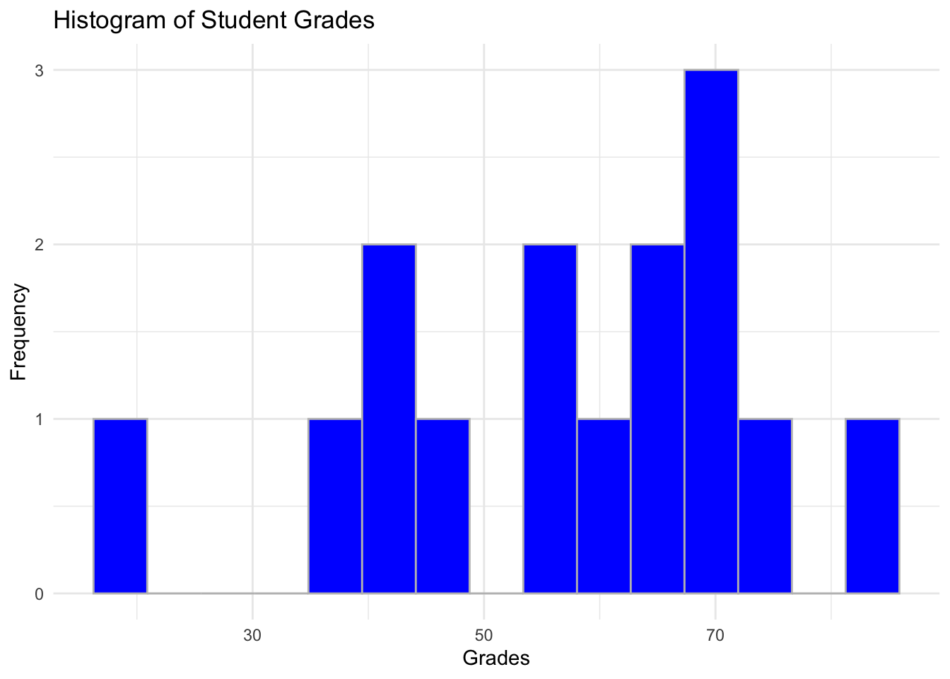
What about by programme? Try plotting with subsets. Bear in mind we don’t have that many observations.
# Example for psych only
ggplot(data = subset(students_grades_prog, programme %in% c('psych')), aes(x = grades)) +
  geom_histogram(bins = 20, color = 'grey', fill = 'blue') +
  labs(x = 'Grades', y = 'Frequency', title = 'Histogram of Student Grades (Psych)') +
  theme_minimal()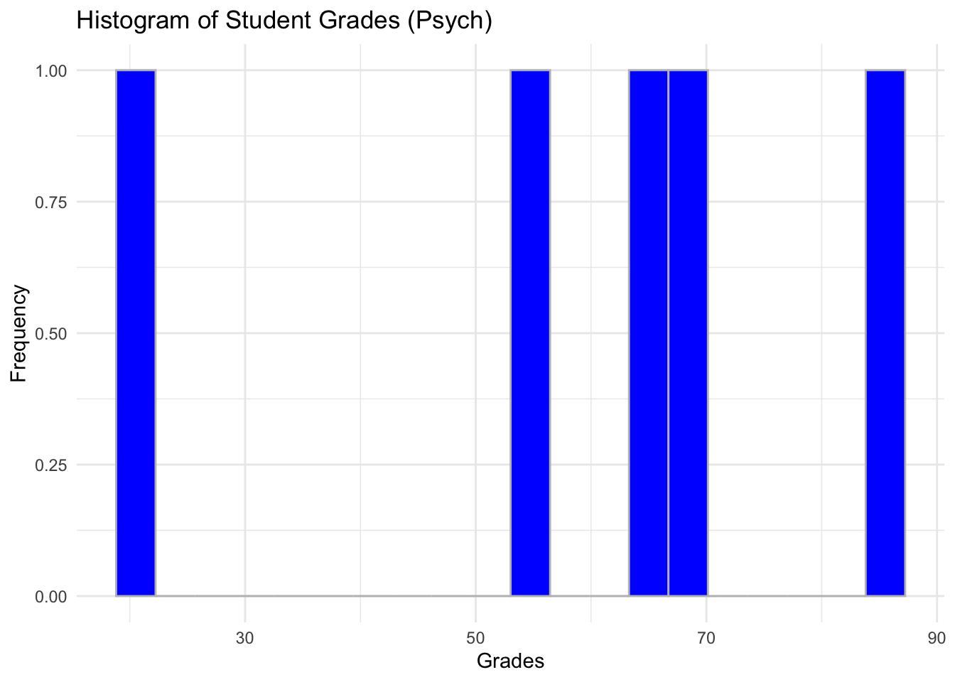
7.10 Save the file in your folder
Before finishing off, we can also write the merged dataset into our folder so it can be saved for the future. Check your folder after you run below.
write.csv(students_grades_prog, 'student_grades_prog.csv') # Note how we first specify the object we want to save and then the name of the file including the extension '.csv'.7.11 Practice.Rmd Solutions
First, make sure that all the necessary packages are loaded:
library(tidyverse)
library(foreign)
For your practice work with the same data as in the tutorial. You will need to use filter and arrange and also mutate to answer the questions below.
You are also required to provide some simple visualisations for your data to show what is happening in student grades by programme.
Here is the breakdown of the tasks we want you to do and the solutions:
- Read all three datasets in (data_students_1, data_students_2, data_students_3). Since they come in different formats make sure to check your notes from the tutorial. Note that you have data_students_3 in different formats so you can choose which one you want to read in. After you’ve read them in, check what’s inside of each dataset.
# Dataset 1
data_students_1 <- read.csv('data_students_1.csv')
head(data_students_1)
## X ID grades
## 1 1 ID_1 20
## 2 2 ID_2 35
## 3 3 ID_3 45
## 4 4 ID_4 85
## 5 5 ID_5 70
## 6 6 ID_6 72# Dataset 2
data_students_2 <- read.table("data_students_2.txt", header = TRUE)
head(data_students_2)## ID programme
## 1 ID_1 psych
## 2 ID_2 lang
## 3 ID_3 phil
## 4 ID_4 psych
## 5 ID_5 lang
## 6 ID_6 phil# Dataset 3
data_students_3 <- read.dta('data_students_3.dta')
head(data_students_3)## ID grades programme
## 1 ID_16 40 psych
## 2 ID_17 38 lang
## 3 ID_18 50 phil
## 4 ID_19 80 psych
## 5 ID_20 69 lang
## 6 ID_21 70 phil# Or
data_students_3 <- read.csv('data_students_3.csv')
head(data_students_3)## X ID grades programme
## 1 1 ID_16 40 psych
## 2 2 ID_17 38 lang
## 3 3 ID_18 50 phil
## 4 4 ID_19 80 psych
## 5 5 ID_20 69 lang
## 6 6 ID_21 70 philNote that we have IDs 16-30 which means that we have got data for an extra 15 students. We can now add these to the other dataset we have. Let us first merge grades and programme for data_students_1 and data_students_2.
- Merge datasets together. First merge data_students_1 and data_students_2, then merge the resulting data with data_students_3. Hint: you will need to use full_join().
# Dataset 1 + Dataset 2
students_grades_prog <- full_join(data_students_1, data_students_2, by = c('ID')) # We can specify the unqiue variable we use to match the datasets via the 'by =' argument.
# + Dataset 3
students_grades_prog_all <- full_join(students_grades_prog, data_students_3) # Please note that we do not need to specify a unique identifier here as we just want to match data by columns and R is clever enough to know what to do.
head(students_grades_prog_all)## X ID grades programme
## 1 1 ID_1 20 psych
## 2 2 ID_2 35 lang
## 3 3 ID_3 45 phil
## 4 4 ID_4 85 psych
## 5 5 ID_5 70 lang
## 6 6 ID_6 72 philWork with the final dataset that has information on all students (30 observations).
Provide means, medians and standard deviations for grades in each programme.
students_grades_prog_all %>%
  group_by(programme) %>%
  summarise(mean = mean(grades),
            median = median(grades),
            sd = sd(grades))
## # A tibble: 3 x 4
## programme mean median sd
## <fct> <dbl> <dbl> <dbl>
## 1 lang 54.7 61 13.8
## 2 phil 56.9 58.5 12.0
## 3 psych 61 65.5 19.1- Provide a simple visualisaiton for each programme.
# Psych
ggplot(data = subset(students_grades_prog_all, programme %in% c('psych')), aes(x = grades)) +
  geom_histogram(bins = 20, color = 'grey', fill = 'cornsilk') +
  labs(x = 'Grades', y = 'Frequency', title = 'Histogram of Student Grades (Psych)') +
  theme_minimal()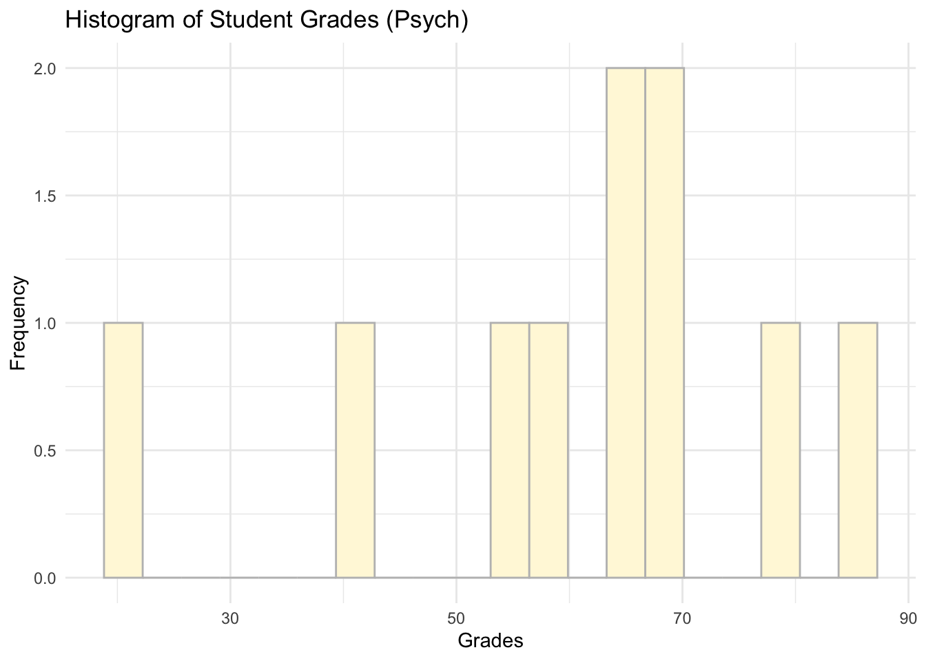
# Lang
ggplot(data = subset(students_grades_prog_all, programme %in% c('lang')), aes(x = grades)) +
  geom_histogram(bins = 20,color = 'grey', fill = 'lightblue') +
  labs(x = 'Grades', y = 'Frequency', title = 'Histogram of Student Grades (Lang)') +
  theme_minimal()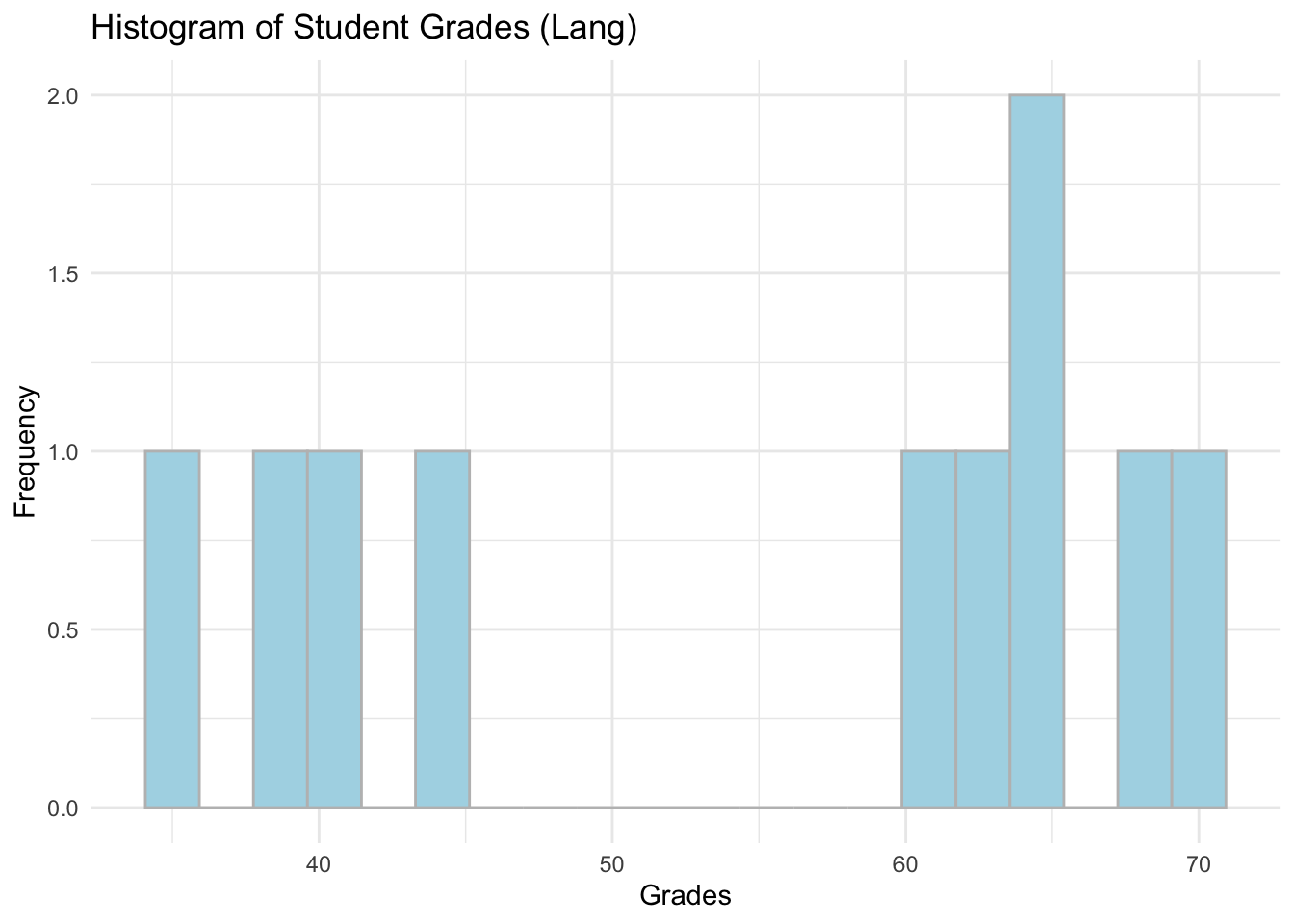
# Phil
ggplot(data = subset(students_grades_prog_all, programme %in% c('phil')), aes(x = grades)) +
  geom_histogram(bins = 20, color = 'grey', fill = 'coral') +
  labs(x = 'Grades', y = 'Frequency', title = 'Histogram of Student Grades (Phil)') +
  theme_minimal()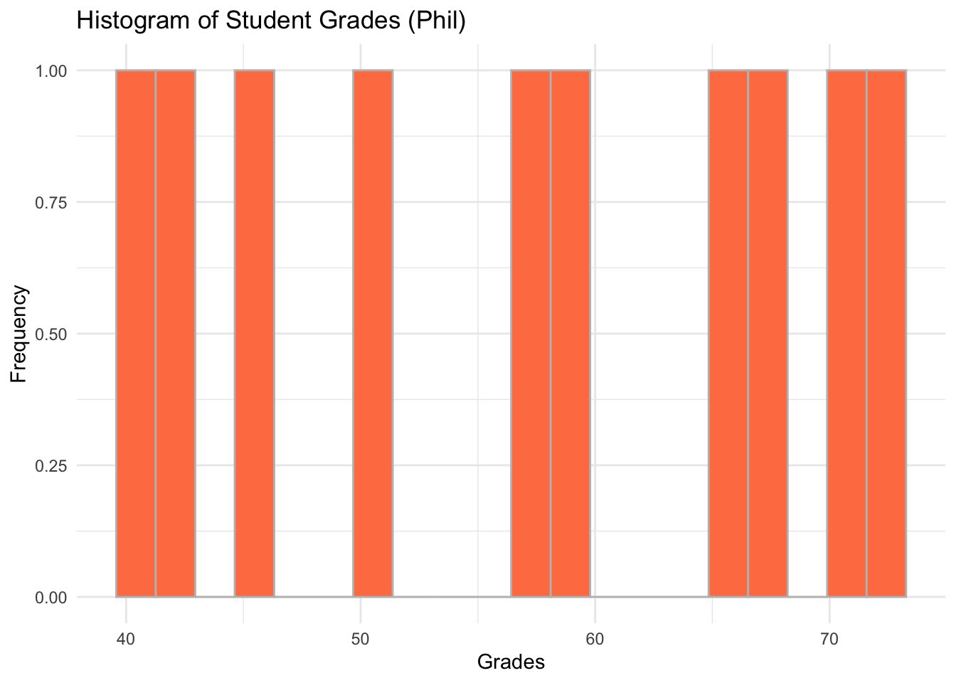
Now, try to answer the following questions:
- How many students in the dataset received the grades above 70?
# Filter for grades above 70
students_grades_prog_all %>%
  filter(grades > 70)
## X ID grades programme
## 1 4 ID_4 85 psych
## 2 6 ID_6 72 phil
## 3 4 ID_19 80 psychThe answer is three.
- What is the mean and the median grade for those who got more than 65?
# Mean and median for grades above 70
students_grades_prog_all %>%
  filter(grades > 65)  %>%
  summarise(mean_above_65 = mean(grades),
            median_above_65 = median(grades))
## mean_above_65 median_above_65
## 1 72 70The answer is 72 and 70.
- How many students received grades that were between 40 and 50 in philosophy programme?
# Phil grades between 40 and 50
students_grades_prog_all %>%
  filter(programme == 'phil') %>%
  filter(grades > 40 & grades < 50) # Note that we use '&' to specify that we want grades both less than 50 and more than 40.
## X ID grades programme
## 1 3 ID_3 45 phil
## 2 15 ID_30 42 philThere are two students.
- Considering only philosophy programme, what were the top three grades in the cohort?
# Only phil arranged
students_grades_prog_all %>%
  filter(programme == 'phil') %>%
  arrange(desc(grades))
## X ID grades programme
## 1 6 ID_6 72 phil
## 2 6 ID_21 70 phil
## 3 12 ID_12 68 phil
## 4 12 ID_27 65 phil
## 5 9 ID_24 59 phil
## 6 9 ID_9 58 phil
## 7 3 ID_18 50 phil
## 8 3 ID_3 45 phil
## 9 15 ID_30 42 phil
## 10 15 ID_15 40 philThe answer is 72, 70 and 68.
- Now, for language, what were the three lowest grades in the cohort?
# Only lang arranged
students_grades_prog_all %>%
  filter(programme == 'lang')  %>%
  arrange(grades)
## X ID grades programme
## 1 2 ID_2 35 lang
## 2 2 ID_17 38 lang
## 3 11 ID_26 40 lang
## 4 11 ID_11 44 lang
## 5 8 ID_8 60 lang
## 6 8 ID_23 62 lang
## 7 14 ID_14 64 lang
## 8 14 ID_29 65 lang
## 9 5 ID_20 69 lang
## 10 5 ID_5 70 langIt should be 35, 38 and 40.
Well done. It may have taken a while to build all of these code chunks but it is an essential part of the practice to keep playing with the code we are showing you. Try to arrange things differently and see what happens.