Chapter 5 Results
library(tidyverse)
library(lubridate)
library(ggplot2)

load("combined_data.RData")
5.1 NDVI Graphs
# Monthly Averages
ndvi_monthavg2 <- aggregate(ndvi ~ month + year + transect + date + wetland + type, compiled_wetlands, mean)

# Freshwater Emergent Graphs
freshwater_wetlands <- c("WestCreek", "Matukat", "GooseCreek")
freshwater_types <- c("Freshwater Emergent")

ndvi_monthavg2 %>%
  filter(wetland %in% freshwater_wetlands, type %in% freshwater_types) %>%
  mutate(date = as.Date(date, format = "%m/%d/%Y")) %>%
  ggplot() +
  geom_line(aes(x = date, y = ndvi, color = transect, group = interaction(wetland, type))) +
  scale_x_date(date_breaks = "60 months", date_labels = "%b-%Y") +
  facet_grid(rows = vars(wetland), cols = vars(type), scales = "free") +
  theme(legend.position = "none") +
  labs(title = "Freshwater Emergent Site Graphs", caption = "Figure 4: Summer monthly averages of NDVI at each transect for Freshwater emergent wetland plots in the Hayman Fire perimeter") +
  theme(plot.caption = element_text(hjust = 0.5))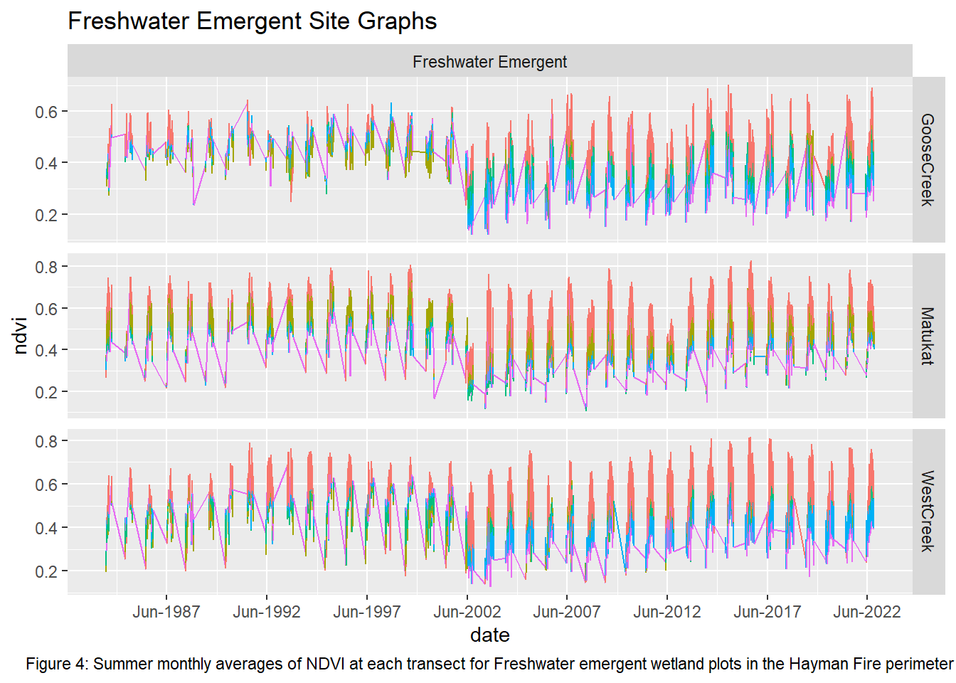
# Forested/Shrub Graphs
forested_wetlands <- c("SHighway", "MatukatShrub", "TurkeyCreek")
forested_types <- c("Shrub Wetland/Forested Freshwater")

ndvi_monthavg2 %>%
  filter(wetland %in% forested_wetlands, type %in% forested_types) %>%
  mutate(date = as.Date(date, format = "%m/%d/%Y")) %>%
  ggplot() +
  geom_line(aes(x = date, y = ndvi, color = transect, group = interaction(wetland, type))) +
  scale_x_date(date_breaks = "60 months", date_labels = "%b-%Y") +
  facet_grid(rows = vars(wetland), cols = vars(type), scales = "free") +
  theme(legend.position = "none") +
  labs(title = "Shrub Wetland/Forested Freshwater Site Graphs", caption = "Figure 5: Summer monthly averages of NDVI at each Shrub Wetland/Forested Freshwater plots in the Hayman Fire perimeter")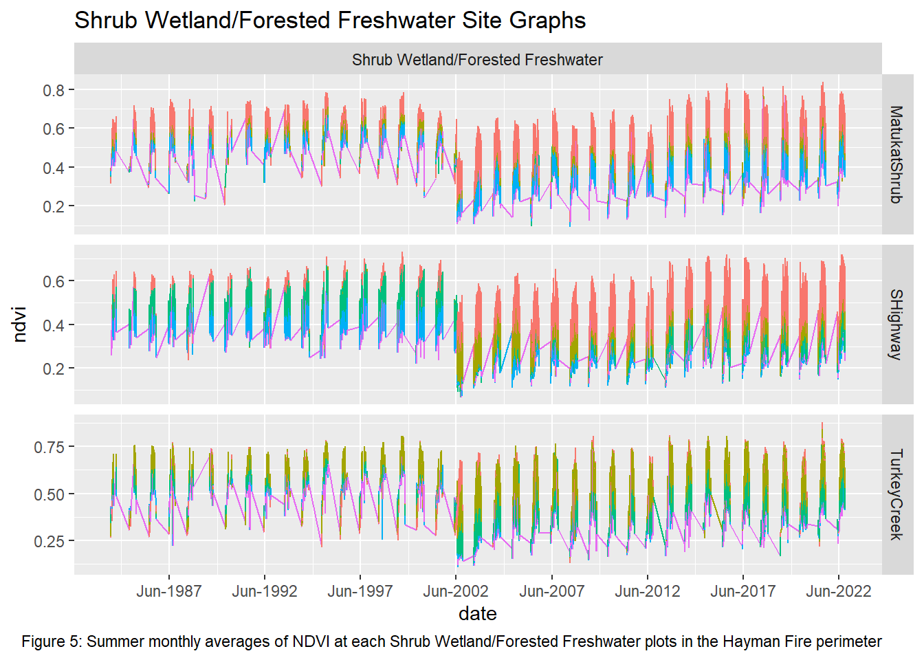
# Non-Wetland Graphs
non_wetlands <- c("FourMile", "TrailCreek", "LongWater")
non_types <- c("Non-Wetland")

ndvi_monthavg2 %>%
  filter(wetland %in% non_wetlands, type %in% non_types) %>%
  mutate(date = as.Date(date, format = "%m/%d/%Y")) %>%
  ggplot() +
  geom_line(aes(x = date, y = ndvi, color = transect, group = interaction(wetland, type))) +
  scale_x_date(date_breaks = "60 months", date_labels = "%b-%Y") +
  facet_grid(rows = vars(wetland), cols = vars(type), scales = "free") +
  theme(legend.position = "none", ) +
  labs(title = "Non-Wetland Site Graphs", caption = "Figure 6: Summer monthly averages of NDVI at each transect for Non-wetland plots in the Hayman Fire perimeter")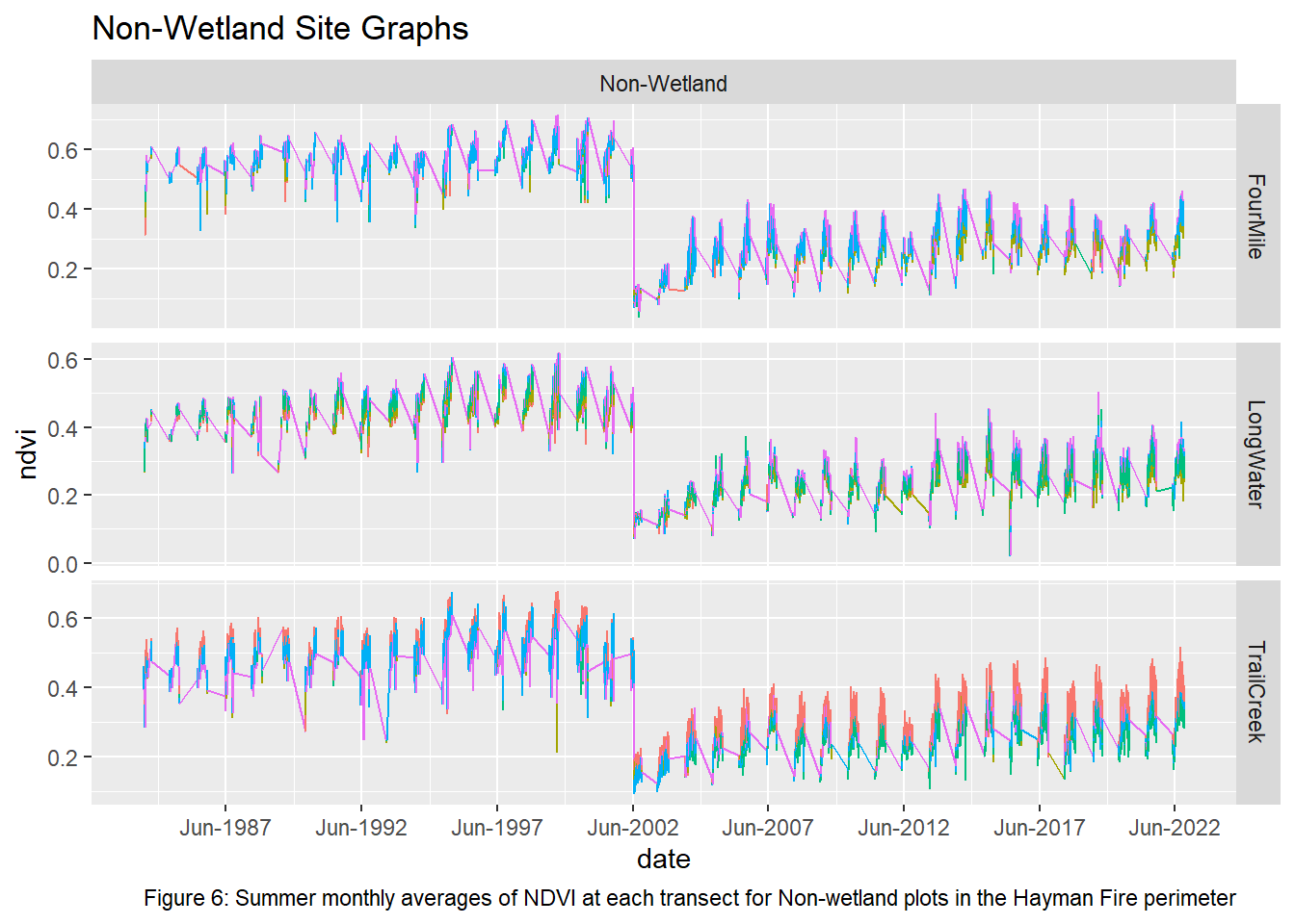
Upon visual examination of the data, there is a clear difference in the recovery rates with all transects from the non-wetland sites not returning to pre-fire greenness in the 20 years since the fire. Both Freshwater Emergent and Shrub/Forested sites have improved recovery rates over the non-wetlands. The first transect for the two wetland types shows that NDVI values did not vary much pre and post fire while the non-wetland sites have drastic differences. However, the second and third transects for the Freshwater Emergent and Shrub/Forested sites show that change occurred from the fire and that the recovery relative to non-wetlands was much quicker. The final transect shows patterns most similar to non-wetlands, indicating wetlands have the least impact on vegetation recovery at around 400 meters away.
5.2 NDVI Transect Graphs
## Position Graphs
# Freshwater
freshwater_transect <- c("0m", "100m", "200m", "300m", "400m")
freshwater_types <- c("Freshwater Emergent")
goosecreek <- c("GooseCreek")

ndvi_monthavg2 %>%
  filter(wetland %in% goosecreek, type %in% freshwater_types, transect %in% freshwater_transect) %>%
  mutate(date = as.Date(date, format = "%m/%d/%Y")) %>%
  ggplot() +
  geom_line(aes(x = date, y = ndvi, color = transect, group = interaction(wetland, type))) +
  scale_x_date(date_breaks = "60 months", date_labels = "%b-%Y") +
  facet_grid(rows = vars(transect), cols = vars(wetland), scales = "free") +
  theme(legend.position = "none", ) +
labs(title = "Goose Creek Transect Graphs", caption = "Figure 7: Summer monthly averages of NDVI of each individual transect at the Goose Creek Freshwater Emergent wetland in the Hayman Fire perimeter") + theme(plot.caption = element_text(size = 10, hjust = 0.5, margin = margin(t = 10))) 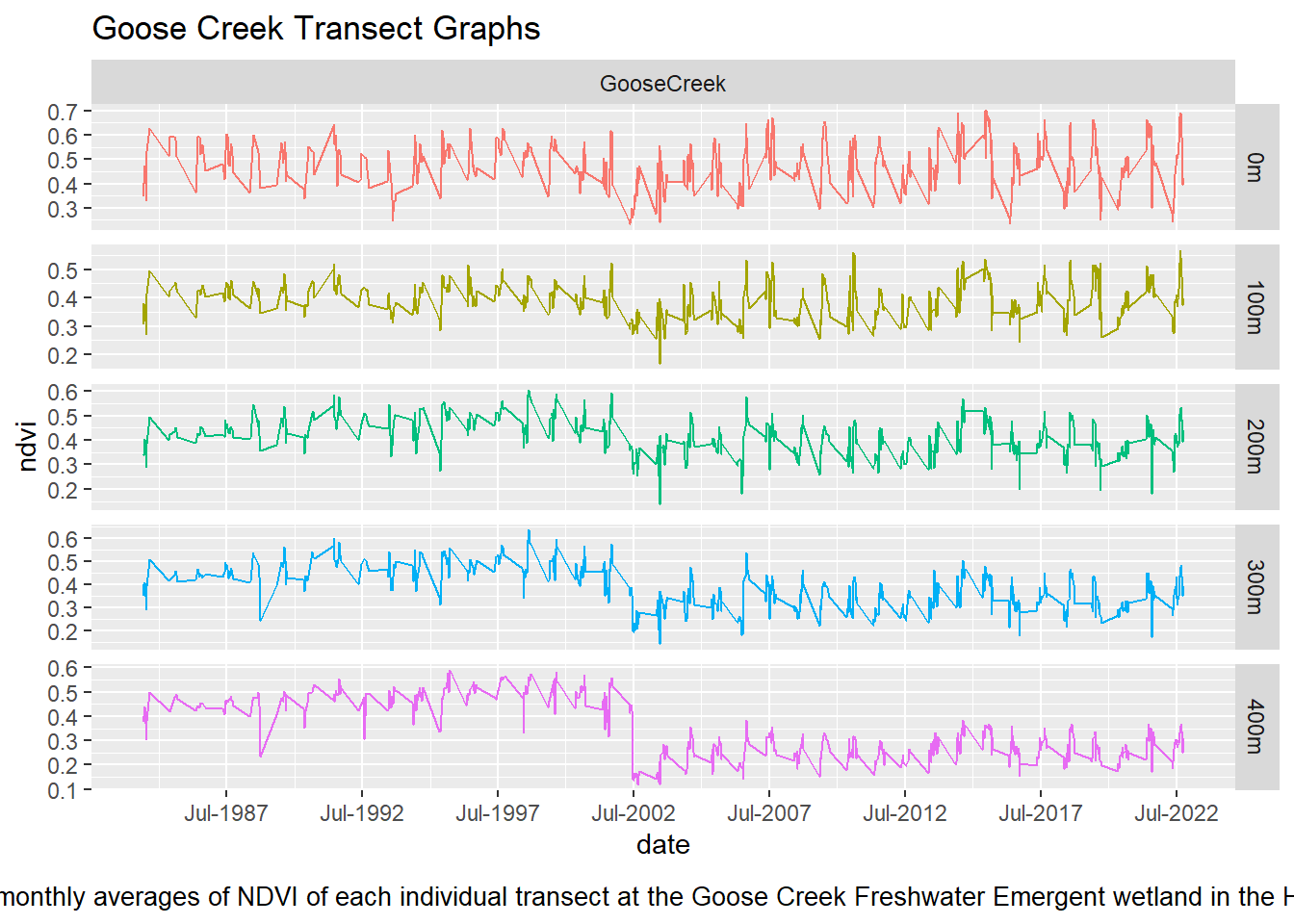
# Forested/Shrub Graphs
forestedshrub_types <- c("Shrub Wetland/Forested Freshwater")
turkeycreek <- c("TurkeyCreek")

ndvi_monthavg2 %>%
  filter(wetland %in% turkeycreek, type %in% forestedshrub_types, transect %in% freshwater_transect) %>%
  mutate(date = as.Date(date, format = "%m/%d/%Y")) %>%
  ggplot() +
  geom_line(aes(x = date, y = ndvi, color = transect, group = interaction(wetland, type))) +
  scale_x_date(date_breaks = "60 months", date_labels = "%b-%Y") +
  facet_grid(rows = vars(transect), cols = vars(wetland), scales = "free") +
  theme(legend.position = "none", ) +
  labs(title = "Turkey Creek Transect Graphs", caption = "Figure 8: Summer monthly averages of NDVI of each individual transect at the Turkey Creek Shrub Wetland/Forested Freshwater in the Hayman Fire perimeter") +
  theme(plot.caption = element_text(hjust = 0.5))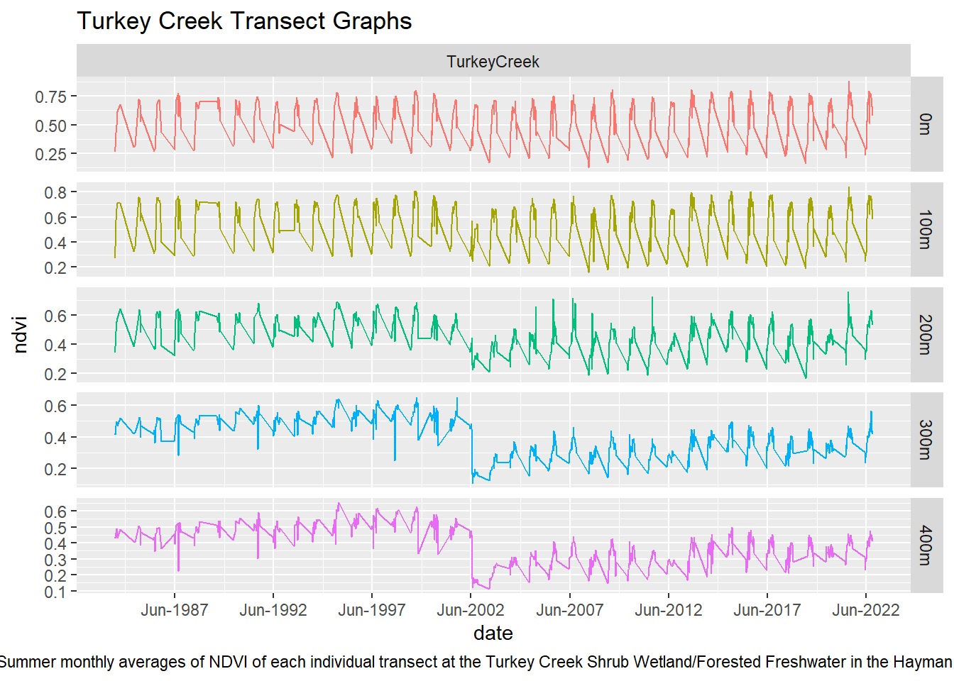
# Non-Wetland
nonwetland_types <- c("Non-Wetland")
trailcreek <- c("TrailCreek")

ndvi_monthavg2 %>%
  filter(wetland %in% trailcreek, type %in% nonwetland_types, transect %in% freshwater_transect) %>%
  mutate(date = as.Date(date, format = "%m/%d/%Y")) %>%
  ggplot() +
  geom_line(aes(x = date, y = ndvi, color = transect, group = interaction(wetland, type))) +
  scale_x_date(date_breaks = "60 months", date_labels = "%b-%Y") +
  facet_grid(rows = vars(transect), cols = vars(wetland), scales = "free") +
  theme(legend.position = "none", ) +
  labs(title = "Trail Creek Transect Graphs", caption = "Figure 9: Summer monthly averages of NDVI of each individual transect at the Trail Creek non-wetland in the Hayman Fire perimeter") +
  theme(plot.caption = element_text(hjust = 0.5))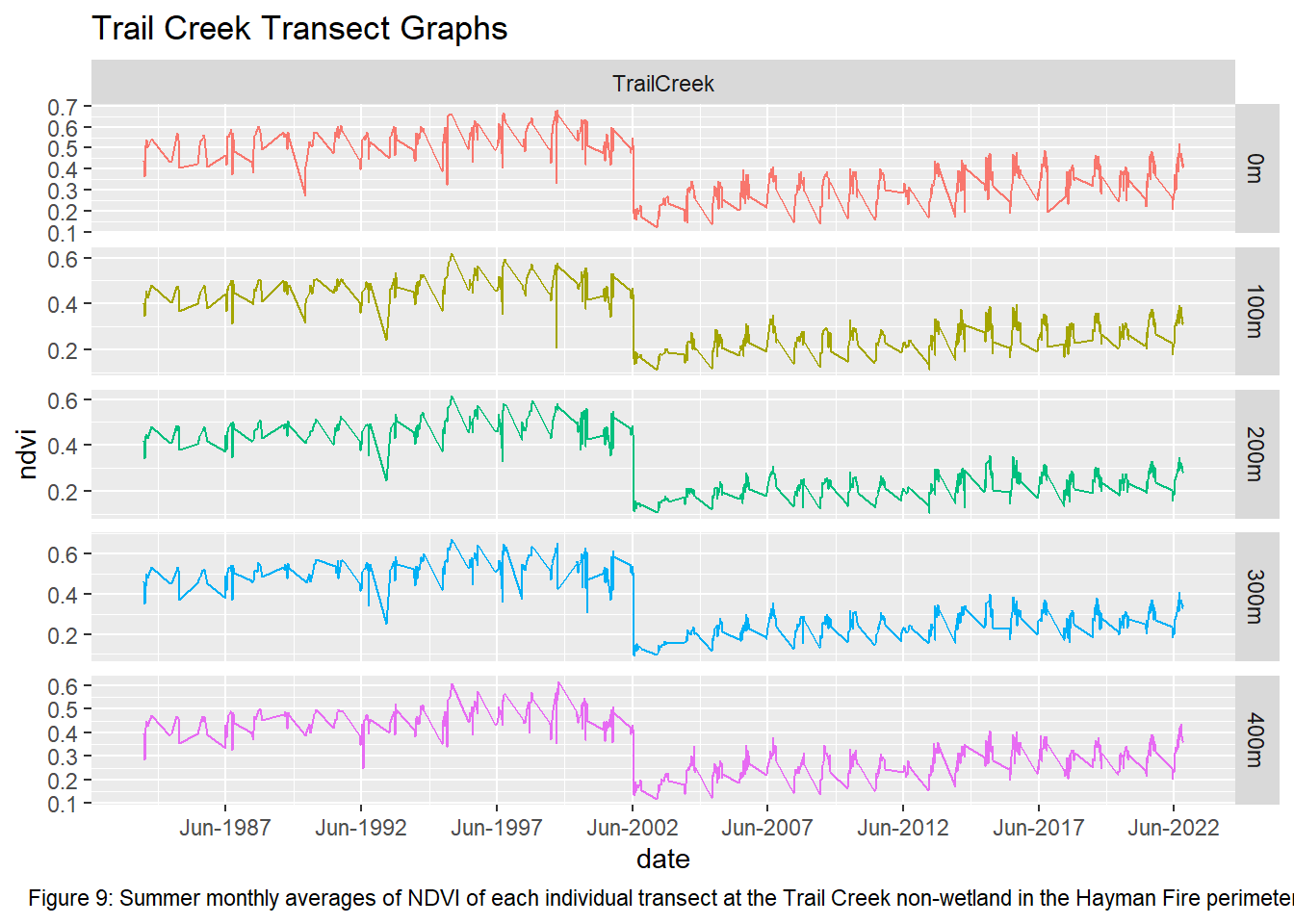
5.3 NDVI ANOVA Data
# Adjustments of previous data
# Yearly Median
ndvi_yearmedian <- aggregate(ndvi ~ year + transect + wetland + type, compiled_wetlands, median)

# Data Post-Fire NDVI
ndvi_yearmedian_postfire <- ndvi_yearmedian %>%
  filter(year >= 2003)

# Type and transect
ndvi_yearmedian_0m <- ndvi_yearmedian_postfire %>%
  filter(transect == "0m")

ndvi_yearmedian_100m <- ndvi_yearmedian_postfire %>%
  filter(transect == "100m")

ndvi_yearmedian_200m <- ndvi_yearmedian_postfire %>%
  filter(transect == "200m")

ndvi_yearmedian_300m <- ndvi_yearmedian_postfire %>%
  filter(transect == "300m")

ndvi_yearmedian_400m <- ndvi_yearmedian_postfire %>%
  filter(transect == "400m")
5.4 ANOVA Test
# # NDVI
# Fit the ANOVA model. Landscape position alters the type of response

# Perform a repeated measures ANOVA
aov_repmeas0m <- aov(ndvi ~ type, data = ndvi_yearmedian_0m)

aov_repmeas100m <- aov(ndvi ~ type, data = ndvi_yearmedian_100m)

aov_repmeas200m <- aov(ndvi ~ type, data = ndvi_yearmedian_200m)

aov_repmeas300m <- aov(ndvi ~ type, data = ndvi_yearmedian_300m)

aov_repmeas400m <- aov(ndvi ~ type, data = ndvi_yearmedian_400m)
# Boxplots of Summer Medians
ggplot(ndvi_yearmedian_0m, aes(x = type, y = ndvi)) +
geom_boxplot() +
xlab("Type") +
ylab("Median NDVI") +
labs(title = "Median Summer NDVI at 0 meter Transect", caption = "Figure 10: Boxplot showing the distribution of the median of summer averages of NDVI values by wetland type for the 0 meter transects") +
theme(plot.caption = element_text(hjust = 0.5))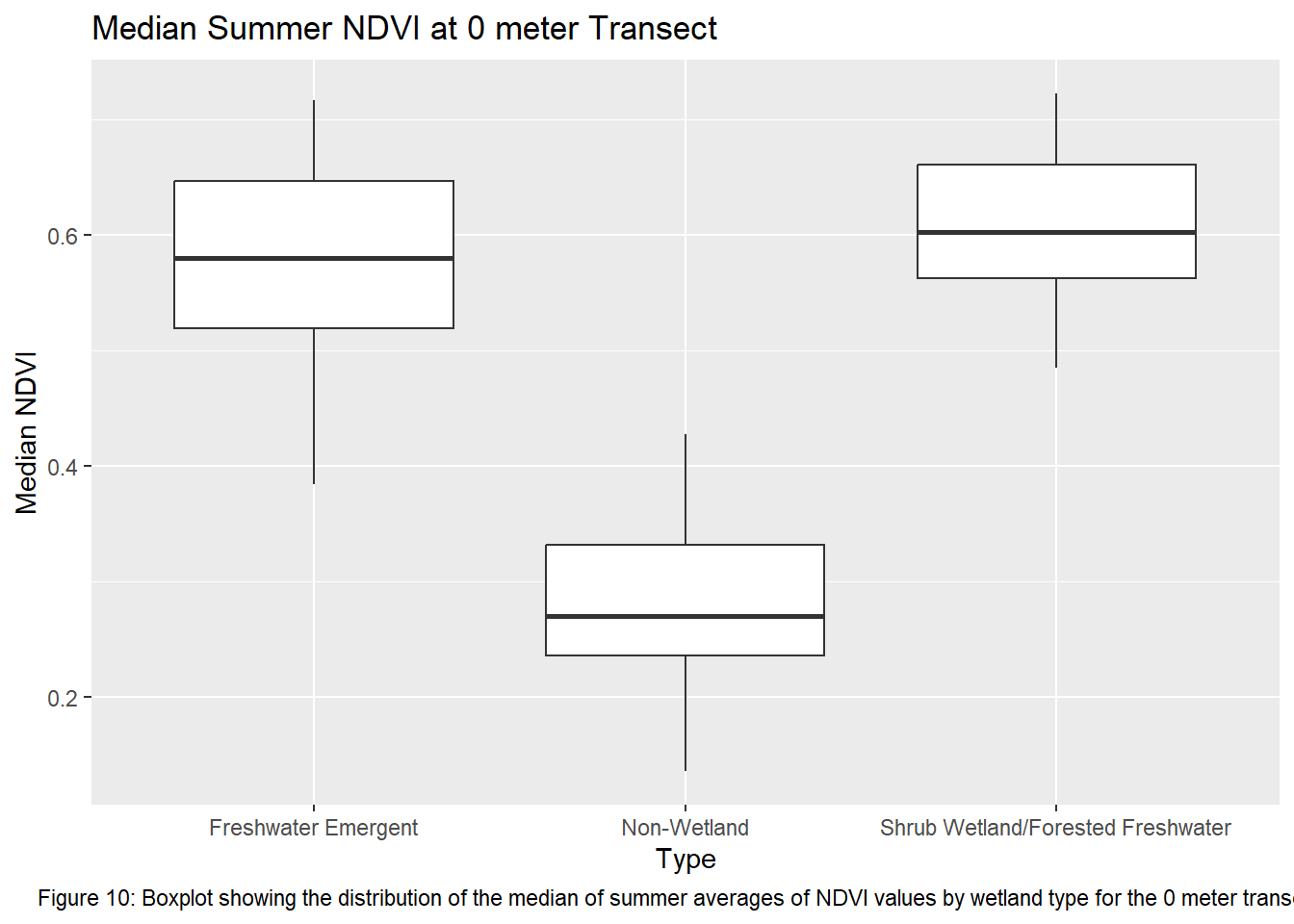
ggplot(ndvi_yearmedian_100m, aes(x = type, y = ndvi)) +
  geom_boxplot() +
  xlab("Type") +
  ylab("Median NDVI") +
  labs(title = "Median Summer NDVI at 100 meter Transect", caption = "Figure 11: Boxplot showing the distribution of the median of summer averages of NDVI values by wetland type for the 100 meter transects") +
  theme(plot.caption = element_text(hjust = 0.5))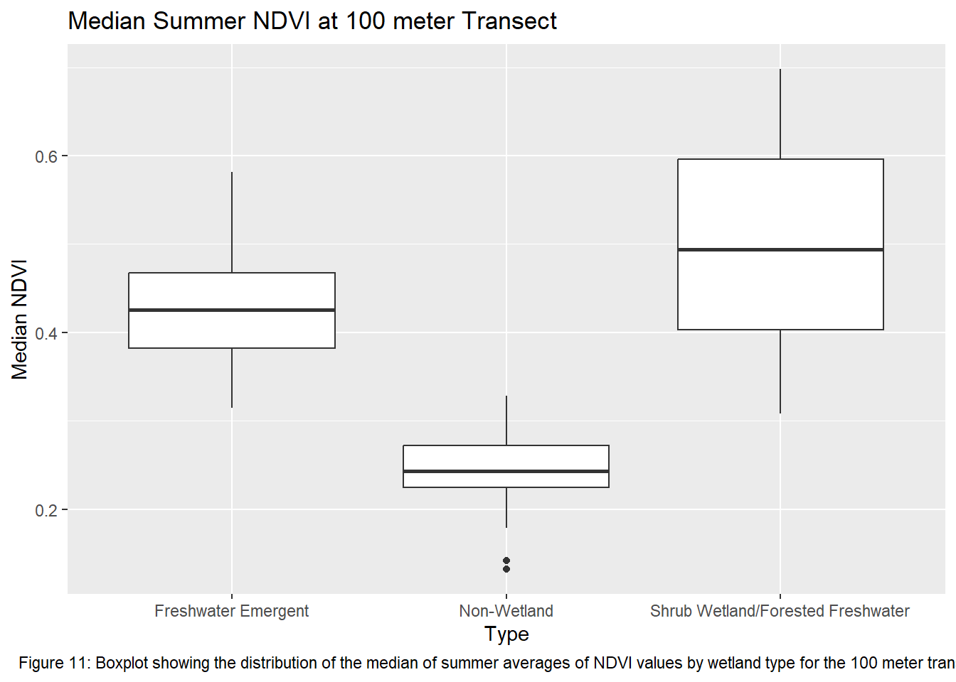
ggplot(ndvi_yearmedian_200m, aes(x = type, y = ndvi)) +
  geom_boxplot() +
  xlab("Type") +
  ylab("Median NDVI") +
  labs(title = "Median Summer NDVI at 200 meter Transect", caption = "Figure 12: Boxplot showing the distribution of the median of summer averages of NDVI values by wetland type for the 200 meter transects") +
  theme(plot.caption = element_text(hjust = 0.5))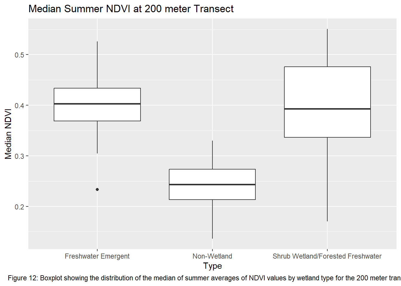
ggplot(ndvi_yearmedian_300m, aes(x = type, y = ndvi)) +
  geom_boxplot() +
  xlab("Type") +
  ylab("Median NDVI") +
  labs(title = "Median Summer NDVI at 300 meter Transect", caption = "Figure 13: Boxplot showing the distribution of the median of summer averages of NDVI values by wetland type for the 300 meter transects") +
  theme(plot.caption = element_text(hjust = 0.5))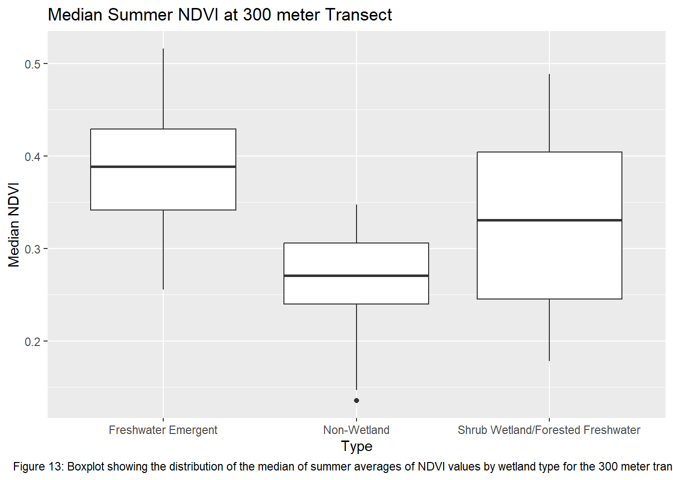
ggplot(ndvi_yearmedian_400m, aes(x = type, y = ndvi)) +
  geom_boxplot() +
  xlab("Type") +
  ylab("Median NDVI") +
  labs(title = "Median Summer NDVI at 400 meter Transect", caption = "Figure 14: Boxplot showing the distribution of the median of summer averages of NDVI values by wetland type for the 400 meter transects") +
  theme(plot.caption = element_text(hjust = 0.5))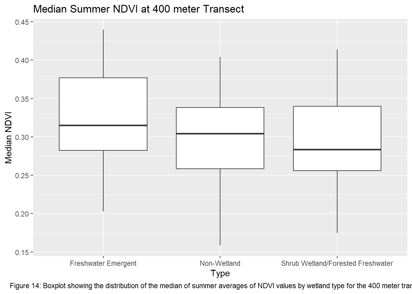
5.5 ANOVA Results
Running the ANOVA tests only further support that wetlands influence vegetation recovery with each transect returning a p-value < 0.05. This indicates that the values between transects for each wetland type are significantly different from one another. Though given the ANOVA is an omnibus test, meaning it’s unclear which wetland types are different from each other, the boxplots of the summer median values show clearly which sites vary most from the others. The use of an auto-regressive integrated moving average (ARIMA) or a first order auto-regressive model would aid in a more comprehensive understanding of the variation occurring between these sites. However, the least amount of variance comes from the farthest transect of each wetland type. At 400 meters the median NDVI values reflect much less variation between wetland types. The ANOVA shows limited variation as it returned the highest p-value of all the transects.
# ANOVA Results
summary(aov_repmeas0m)
## Df Sum Sq Mean Sq F value Pr(>F)
## type 2 3.894 1.9471 383.7 <2e-16 ***
## Residuals 177 0.898 0.0051
## ---
## Signif. codes: 0 '***' 0.001 '**' 0.01 '*' 0.05 '.' 0.1 ' ' 1summary(aov_repmeas100m)## Df Sum Sq Mean Sq F value Pr(>F)
## type 2 2.000 1.0002 152 <2e-16 ***
## Residuals 177 1.165 0.0066
## ---
## Signif. codes: 0 '***' 0.001 '**' 0.01 '*' 0.05 '.' 0.1 ' ' 1summary(aov_repmeas200m)## Df Sum Sq Mean Sq F value Pr(>F)
## type 2 0.9584 0.4792 108.7 <2e-16 ***
## Residuals 177 0.7803 0.0044
## ---
## Signif. codes: 0 '***' 0.001 '**' 0.01 '*' 0.05 '.' 0.1 ' ' 1summary(aov_repmeas300m)## Df Sum Sq Mean Sq F value Pr(>F)
## type 2 0.4484 0.22418 47.44 <2e-16 ***
## Residuals 177 0.8364 0.00473
## ---
## Signif. codes: 0 '***' 0.001 '**' 0.01 '*' 0.05 '.' 0.1 ' ' 1summary(aov_repmeas400m)## Df Sum Sq Mean Sq F value Pr(>F)
## type 2 0.0295 0.014751 4.723 0.01 *
## Residuals 177 0.5528 0.003123
## ---
## Signif. codes: 0 '***' 0.001 '**' 0.01 '*' 0.05 '.' 0.1 ' ' 1library(broom)
library(dplyr)
aov_results <- bind_rows(
tidy(aov_repmeas0m),
tidy(aov_repmeas100m),
tidy(aov_repmeas200m),
tidy(aov_repmeas300m),
tidy(aov_repmeas400m)
)
aov_results## # A tibble: 10 × 6
## term df sumsq meansq statistic p.value
## <chr> <dbl> <dbl> <dbl> <dbl> <dbl>
## 1 type 2 3.89 1.95 384. 4.38e-65
## 2 Residuals 177 0.898 0.00507 NA NA
## 3 type 2 2.00 1.00 152. 3.78e-39
## 4 Residuals 177 1.16 0.00658 NA NA
## 5 type 2 0.958 0.479 109. 1.61e-31
## 6 Residuals 177 0.780 0.00441 NA NA
## 7 type 2 0.448 0.224 47.4 3.18e-17
## 8 Residuals 177 0.836 0.00473 NA NA
## 9 type 2 0.0295 0.0148 4.72 1.00e- 2
## 10 Residuals 177 0.553 0.00312 NA NA