3 Essential Algebra and Set Theory
In this chapter we review many components of Isabelle’s Main library that
are ubiquitous everywhere else. Learning this will make you familiar with basic
concepts from abstract algebra and set theory. Feel free to skip this chapter and come back to
individual sections as necessary.
3.1 Order
3.1.1 Motivation of order axioms
We take it for granted that numbers are ordered. For example we know that no matter which two numbers
we pick, one of them must be greater or equal to the other.
For all x and y, either x ≤ y or y ≤ x.
For Isabelle this is not so obvious.
What does ≤ even mean? For example we could intuitively agree that the empty set
{} is smaller than {1}, which in turn is “obviously” smaller than {1,2}.
The set {2} is also greater than {} and {1,2}. In Isabelle we can write is as
value "{1} ≤ ({1,2}::nat set)" (* prints "True" *)
value "{2} ≤ ({1,2}::nat set)" (* prints "True" *)
value "{} ≤ ({1}::nat set)" (* prints "True" *)
value "{} ≤ ({2}::nat set)" (* prints "True" *)
What about comparing {1} with {2}?
value "{1} ≤ ({2}::nat set)" (* prints "False" *)
value "{2} ≤ ({1}::nat set)" (* prints "False" *)
This violates the rule that so “obviously” held for numbers
linear: "x ≤ y ∨ y ≤ x"We also intuitively know that if x ≤ y and y ≤ x then x=y.
order_antisym : "x ≤ y ⟹ y ≤ x ⟹ x = y"There are certain mathematical objects that violate order_antisym too. For example
consider any ranking board where players are ordered by the number of points they scored.
Two players may have equal score but that doesn’t mean they are the same person.
3.1.2 Order type classes
Isabelle defines an entire hierarchy of type classes that
correspond to different orders. The first one is ord which only defines two predicates
less_eq and less but does not assume any axioms. The sole purpose of this class
is to introduce syntactic sugar.
(* Use this line to avoid conflicts with Main*)
no_notation less_eq  ("'(≤')") and less_eq  ("(_/ ≤ _)"  [51, 51] 50) and  less  ("'(<')") and  less  ("(_/ < _)"  [51, 51] 50) and greater_eq (infix "≥" 50) and greater  (infix ">" 50)

class ord =
  fixes less_eq :: "'a ⇒ 'a ⇒ bool"
    and less :: "'a ⇒ 'a ⇒ bool"
begin

notation
  less_eq  ("'(≤')") and
  less_eq  ("(_/ ≤ _)"  [51, 51] 50) and
  less  ("'(<')") and
  less  ("(_/ < _)"  [51, 51] 50)

abbreviation (input)
  greater_eq  (infix "≥" 50)
  where "x ≥ y ≡ y ≤ x"

abbreviation (input)
  greater  (infix ">" 50)
  where "x > y ≡ y < x"

notation (ASCII)
  less_eq  ("'(<=')") and
  less_eq  ("(_/ <= _)" [51, 51] 50)

notation (input)
  greater_eq  (infix ">=" 50)

end
The command abbreviation defines a new notation for an arbitrary expression.
A programmer might call this a “macro”. The input and ASCII in brackets specify Isabelle mode
(many unicode symbols have their ASCII counterparts that are easier to type).
A more interesting class is preorder which assumes reflexivity and transitivity
class preorder = ord +
  assumes less_le_not_le: "x < y ⟷ x ≤ y ∧ ¬ (y ≤ x)"
  and order_refl [iff]: "x ≤ x"
  and order_trans: "x ≤ y ⟹ y ≤ z ⟹ x ≤ z"
begin
 (* Here is a bunch of properties that follow from axioms *)
end
The axiom less_le_not_le is necessary because it specifies how less_eq and less predicates are related to one another. Preorder is the most general notion of order that encompasses all of the examples before. We can already use it to prove many simple but useful properties. I have omitted them to keep the definition concise. You can find them in Orderings.thy in Main (using Query or Ctrl+Click 2.4.1).
Now we finally reach partial order.
class order = preorder +
  assumes order_antisym: "x ≤ y ⟹ y ≤ x ⟹ x = y"
begin
    (* lots of theorems *)
end
It includes the law of anti-symmetry. It means that we will never encounter such paradoxes
where two different elements have been assigned the same “spot” in the ordering. A notable example of partially ordered object is 'a set.
The final class is total order which additionally states that all
elements can be compared. Types such as nat and int are totally ordered.
class linorder = order +
  assumes linear: "x ≤ y ∨ y ≤ x"
begin
    (* lots of theorems *)
end
Mathematicians usually refer to ≤ as (total/partial) order and to < as strict (total/partial) order.
The axioms of strict order are derived from axioms of order by applying less_le_not_le axiom.
The following lemma is a statement to that
lemma order_strictI:
  fixes less (infix "<" 50)
    and less_eq (infix "≤" 50)
  assumes "⋀a b. a ≤ b ⟷ a < b ∨ a = b"  (*axiom serving same purpose as less_le_not_le *)
  assumes "⋀a b. a < b ⟹ ¬ b < a" (* assymetry instead of anti-symmetry*)
  assumes "⋀a. ¬ a < a" (* irreflexivity instead of reflexivity *)
  assumes "⋀a b c. a < b ⟹ b < c ⟹ a < c" (*transitivity*)
  shows "class.order less_eq less" (* This is order where predicates less_eq and less switched places *)
  by (rule ordering_orderI) (rule ordering_strictI, (fact assms)+)
If you place your cursor at the end of shows "class.order less_eq less" you will see the following goal
1. class.order (≤) (<)After apply(unfold class.order_def) it becomes
1. class.preorder (≤) (<) ∧ class.order_axioms (≤)After apply(unfold class.preorder_def) and apply(unfold class.order_axioms_def) we arrive at
this convoluted expression
1. ((∀x y. (x < y) = (x ≤ y ∧ ¬ y ≤ x)) ∧ (∀x. x ≤ x) ∧ (∀x y z. x ≤ y ⟶ y ≤ z ⟶ x ≤ z)) ∧
    (∀x y. x ≤ y ⟶ y ≤ x ⟶ x = y)
If we simplify it using apply(auto) we see more clearly the axioms.
 1. ⋀x y. x < y ⟹ x ≤ y
 2. ⋀x y. x < y ⟹ y ≤ x ⟹ False
 3. ⋀x y. x ≤ y ⟹ ¬ y ≤ x ⟹ x < y
 4. ⋀x. x ≤ x
 5. ⋀x y z. x ≤ y ⟹ y ≤ z ⟹ x ≤ z
 6. ⋀x y. x ≤ y ⟹ y ≤ x ⟹ x = y
We can therefore tell that class.order is itself a function that takes two predicates and produces a set of axioms.
What order_strictI shows is that if you swap those two predicates you transform those axioms into different but equivalent ones that correspond to strict order.
Having defined order we can now introduce two functions min and max. They are so simple that we do not need to use primrec nor fun because there is no need for recursion at all. In such cases we can use definition.
definition (in ord) min :: "'a ⇒ 'a ⇒ 'a" where
  "min a b = (if a ≤ b then a else b)"

definition (in ord) max :: "'a ⇒ 'a ⇒ 'a" where
"max a b = (if a ≤ b then b else a)"(in ord) means that those functions are only available for types 'a that instantiate ord.
Click to see an equivalent code example
The notation (in ord) is equivalent to writing the following
class ord =
  fixes less_eq :: "'a ⇒ 'a ⇒ bool"
    and less :: "'a ⇒ 'a ⇒ bool"
begin
  (* ... lemmas ... *)
  definition min :: "'a ⇒ 'a ⇒ 'a" where
    "min a b = (if a ≤ b then a else b)"

  definition  max :: "'a ⇒ 'a ⇒ 'a" where
    "max a b = (if a ≤ b then b else a)"
end
3.1.3 Instantiating fun
Functions are partially ordered.
For example f(x)=2*x is “obviously” greater than g(x)=x because
g(x) ≤ f(x)for all x. This is proved as follows.
(* an auxiliary lemma similar to Nat.nat_mult_1:"1 * x = x" *)
lemma mul_1_I : "(x::nat) = 1 * x" by (rule sym, rule Nat.nat_mult_1)

theorem "(λ x::nat . x) ≤ (λ x::nat . 2*x)"
  apply(rule le_funI) (* goal: "⋀x. x ≤ 2 * x" *)
  apply(subst mul_1_I) (* goal: "⋀x. 1 * x ≤ 2 * x" *)
  apply(rule mult_le_mono1) (* goal: "⋀x. 1 ≤ 2", mult_le_mono1: "i ≤ j ⟹ i*k ≤ j*k" *)
  apply(simp)
  done
The instantiation of ord for function type 'a ⇒ 'b (also denoted by 'a 'b fun)
is as follows
instantiation "fun" :: (type, ord) ord
begin

definition
  le_fun_def: "f ≤ g ⟷ (∀x. f x ≤ g x)"

definition
  "(f::'a ⇒ 'b) < g ⟷ f ≤ g ∧ ¬ (g ≤ f)"

instance ..

end
The preorder and order do not introduce and new operations so instantiating them
only requires proofs of a few axioms. This can be done as follows.
instance "fun" :: (type, preorder) preorder proof
qed (auto simp add: le_fun_def less_fun_def
  intro: order_trans order.antisym)

instance "fun" :: (type, order) order proof
qed (auto simp add: le_fun_def intro: order.antisym)
3.2 Lattices
3.2.1 Motivation of Lattices
Lattices play major role in Boolean algebra, which in turn is a basis that we will need to work with topology, measure theory and later on probability, real analysis and so on.
We mentioned that 'a set is not totally ordered and instead only follows partial order class order.If we attempted to draw a graph of all elements that are less or equal some set {x,y,z}, we would see the following.
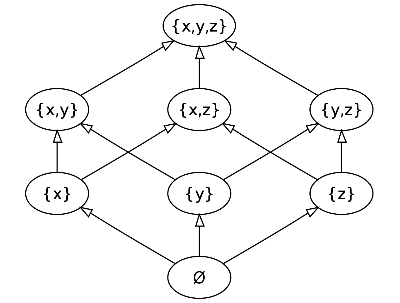
lattice
The empty set is the least element. Every other set is greater than it. Similarly the set {x,y,z} is the greatest element.
By taking the intersection of two sets we can find their greatest common ancestor in the graph. The union of two sets gives us their least common descendant.
For example {x,y} ∩ {x,z} = {x} and {z} ∪ {x} = {x,z} (∩ is written \u, ∪ is \i).
A similar pattern applies to totally ordered set of nat numbers. The minimum of two nat’s yields their greatest lower bound. Maximum yields least upper bound. For example max 3 5 = 5 and min 3 5 = 3.
Lattices allow us to generalize this pattern by introducing two operations called meet ∧ (/\ in ASCII) and join ∨ (\/). In the case of nat, minimum is meet and maximum is join. Notice that ∧ and ∨ are also logical conjunction and disjunction, then
theorem "max x (y::nat) = z ⟹ z ≥ x ∧ z ≥ y"
  by auto

theorem "max x (y::nat) = z ⟹ z ≤ x ∨ z ≤ y"
  by auto

theorem "min x (y::nat) = z ⟹ z ≥ x ∨ z ≥ y"
  by auto

theorem "min x (y::nat) = z ⟹ z ≤ x ∧ z ≤ y"
  by auto
In the case of 'a set, intersection ∩ is meet ∧ and union ∪ is join ∨.
theorem "x ∪ y = {z. z ∈ x ∨ z ∈ y}"
  by auto

theorem "x ∩ y = {z. z ∈ x ∧ z ∈ y}"
  by auto
Therefore, nat is a lattice, 'a set is a lattice and Boolean logic is also a lattice.
In order to avoid confusing meet and join with conjunction and disjunction,
there is also an alternative notation. Meet can be written as ⊓, join as ⊔.
Meet and join are names of the algebraic operations, just like plus is the name of +.
However, the values produced by using these operations are called infimum (for meet) and
supremum (for join), just like the result of x+y is called a sum. Infimum and supremum
are shorter synonyms for greatest lower bound and least upper bound.
Isabelle uses ⊓ and ⊔ notation instead of ∧ and ∨.
3.2.2 Semilattices in Isabelle
The definition of lattices in Isabelle follows a similar philosophy as orders. First we introduce type classes which define the operations of infimum and supremum but don’t provide any axioms.
class inf =
  fixes inf :: "'a ⇒ 'a ⇒ 'a" (infixl "⊓" 70)

class sup =
  fixes sup :: "'a ⇒ 'a ⇒ 'a" (infixl "⊔" 65)
Next we define two “halves” of a lattice (called semilattice)
class semilattice_inf = order + inf +
  assumes inf_le1 [simp]: "x ⊓ y ≤ x"
  and inf_le2 [simp]: "x ⊓ y ≤ y"
  and inf_greatest: "x ≤ y ⟹ x ≤ z ⟹ x ≤ y ⊓ z"

class semilattice_sup = order + sup +
  assumes sup_ge1 [simp]: "x ≤ x ⊔ y"
  and sup_ge2 [simp]: "y ≤ x ⊔ y"
  and sup_least: "y ≤ x ⟹ z ≤ x ⟹ y ⊔ z ≤ x"
begin
(* You might get an error here if you copy-paste this code. Explanation under "Watch out!!" button below. *)
lemma dual_semilattice: "class.semilattice_inf sup greater_eq greater"
  by (rule class.semilattice_inf.intro, rule dual_order)
    (unfold_locales, simp_all add: sup_least)

end
It is a partially ordered (order) type equipped with only one of the two operations.
The axioms inf_le1 and inf_le2 (sup_ge1 and sup_ge2) ensure that the element x ⊓ y (x ⊔ y) is lesser (greater) than any of the elements x and y. Axiom inf_greatest (sup_least) says that there is no fourth element that is in-between all three.
The lemma dual_semilattice is the most interesting. To find out what it means, let us unfold the definitions
lemma dual_semilattice: "class.semilattice_inf sup greater_eq greater"
  apply(unfold class.semilattice_inf_def)
  apply(unfold class.semilattice_inf_axioms_def)
  apply(rule conjI) defer (* defer switches order of subgoals *)
  apply(rule conjI) defer
  apply(rule conjI)
which yields 4 goals
 1. ∀x y. y ≤ sup x y
 2. ∀x y z. y ≤ x ⟶ z ≤ x ⟶ sup y z ≤ x
 3. class.order (λx y. y ≤ x) (λx y. y < x)
 4. ∀x y. x ≤ sup x y
Also by searching for name: semilattice_inf_def (and name: semilattice_sup_def) in Query > Find Theorem tab we get
Lattices.class.semilattice_inf_def:
    Lattices.class.semilattice_inf ?inf ?less_eq ?less ≡
    class.order ?less_eq ?less ∧ Lattices.class.semilattice_inf_axioms ?inf ?less_eq
Lattices.class.semilattice_sup_def:
    Lattices.class.semilattice_sup ?sup ?less_eq ?less ≡
    class.order ?less_eq ?less ∧ Lattices.class.semilattice_sup_axioms ?sup ?less_eq
Watch out!!
If you’re trying to copy this code and experiment on your own you might come across this error
Type unification failed: No type arity bool :: sup

Failed to meet type constraint:

Term:  (⊔) :: ??'a ⇒ ??'a ⇒ ??'a
Type:  bool ⇒ bool ⇒ bool
This is because Isabelle might swap the order of arguments.
Playground.class.semilattice_inf_def:
    Playground.class.semilattice_inf ?less_eq ?less ?inf ≡
    class.order ?less_eq ?less ∧ Playground.class.semilattice_inf_axioms ?less_eq ?inf
The fix is to make sure that the order matches again.
lemma dual_semilattice: "class.semilattice_inf greater_eq greater sup"Therefore, the lemma dual_semilattice states that if we apply to sup greater_eq greater to Lattices.class.semilattice_inf ?inf ?less_eq ?less we obtain a valid lattice. Visually it means that we flip the lattice upside-down. Top element becomes bottom one and vice-versa. Meet becomes join. Less than becomes greater than. Such flipped lattice is called dual.
3.2.3 Lattices in Isabelle
Infimum semilattice allows us to find “minimum” of two elements but we have no means of finding the “maximum” one. Supremum semilattice has the opposite problem. Therefore, let us define lattice
class lattice = semilattice_inf + semilattice_supas an object equipped with both meet and join. A similar duality holds here as well.
context lattice
begin

lemma dual_lattice: "class.lattice sup (≥) (>) inf"
  by (rule class.lattice.intro,
      rule dual_semilattice,
      rule class.semilattice_sup.intro,
      rule dual_order)
    (unfold_locales, auto)

end
Notice that dual_semilattice was proved in a begin and end scope that followed directly after definition of semilattice_sup type class. This time, dual_lattice is defined within context lattice. The two notations are equivalent.
Example
class semilattice_sup = order + sup +
  assumes sup_ge1 [simp]: "x ≤ x ⊔ y"
  and sup_ge2 [simp]: "y ≤ x ⊔ y"
  and sup_least: "y ≤ x ⟹ z ≤ x ⟹ y ⊔ z ≤ x"

(* you can put some code in between or you could even move dual_semilattice to a different file *)

context semilattice_sup
begin

lemma dual_semilattice: "class.semilattice_inf greater_eq greater sup"
  by (rule class.semilattice_inf.intro, rule dual_order)
    (unfold_locales, simp_all add: sup_least)

end
We are going to now state several important algebraic properties of lattices but we
will omit the proofs. They are left as an exercise or can be found in Main library.
lemma dual_lattice: "class.lattice sup (≥) (>) inf"

lemma inf_sup_absorb [simp]: "x ⊓ (x ⊔ y) = x"

lemma sup_inf_absorb [simp]: "x ⊔ (x ⊓ y) = x"

lemma distrib_sup_le: "x ⊔ (y ⊓ z) ≤ (x ⊔ y) ⊓ (x ⊔ z)"

lemma distrib_inf_le: "(x ⊓ y) ⊔ (x ⊓ z) ≤ x ⊓ (y ⊔ z)"

lemma distrib_imp1:
  assumes distrib: "⋀x y z. x ⊓ (y ⊔ z) = (x ⊓ y) ⊔ (x ⊓ z)"
  shows "x ⊔ (y ⊓ z) = (x ⊔ y) ⊓ (x ⊔ z)"

lemma distrib_imp2:
  assumes distrib: "⋀x y z. x ⊔ (y ⊓ z) = (x ⊔ y) ⊓ (x ⊔ z)"
  shows "x ⊓ (y ⊔ z) = (x ⊓ y) ⊔ (x ⊓ z)"
The last two of them work only if you assume distrib (distributivity). It is such an important case
that it deserved its own type class
class distrib_lattice = lattice +
  assumes sup_inf_distrib1: "x ⊔ (y ⊓ z) = (x ⊔ y) ⊓ (x ⊔ z)"
3.3 Top and bottom
3.3.1 Type classes
Bottom is an element ⊥ such that every other a is greater or equal ⊥.
class bot =
  fixes bot :: 'a ("⊥")

class order_bot = order + bot +
  assumes bot_least: "⊥ ≤ a"
For example nat has 0 as bottom
value "bot::nat"
(* prints "0" *)
and set has {} as bottom
value "bot::nat set"
(* prints "{}" *)
Remark: if all types are inhabited how can we have empty set?
We mentioned before (2.6.3) that all types in Isabelle are inhabited and therefore we have theundefined axiom. So you might be wondering how is it possible that we have an empty set? The answer is simple. Empty set is an element of type set. Only types must be inhabited. Empty set {} is the proof that 'a set is inhabited for all types 'a.
Analogically the top element ⊤ is the greatest one.
class top =
  fixes top :: 'a ("⊤")

class order_top = order + top +
  assumes top_greatest: "a ≤ ⊤"
A lattice endowed with top or bottom element is defined as bounded lattice
class bounded_lattice_top = lattice + order_top

class bounded_lattice_bot = lattice + order_bot

class bounded_lattice = lattice + order_bot + order_top
Key properties of top and bottom are
lemma inf_bot_left [simp]: "⊥ ⊓ x = ⊥"

lemma inf_bot_right [simp]: "x ⊓ ⊥ = ⊥"

lemma sup_top_left [simp]: "⊤ ⊔ x = ⊤"

lemma sup_top_right [simp]: "x ⊔ ⊤ = ⊤"
3.3.2 Instantiating fun
Let us use function type as an the example again (3.1.3). The bottom function is a constant function that returns the bottom element of its domain. Analogically for top.
instantiation "fun" :: (type, bot) bot
begin

definition
  "⊥ = (λx. ⊥)" (* recall that λ (written `\l`) is an anonymous function (also known as lambda expression) *)

instance ..

end

instantiation "fun" :: (type, order_bot) order_bot
begin

lemma bot_apply [simp, code]:
  "⊥ x = ⊥"
  by (simp add: bot_fun_def)

instance proof
qed (simp add: le_fun_def)

end

instantiation "fun" :: (type, top) top
begin

definition
  [no_atp]: "⊤ = (λx. ⊤)"

instance ..

end

instantiation "fun" :: (type, order_top) order_top
begin

lemma top_apply [simp, code]:
  "⊤ x = ⊤"
  by (simp add: top_fun_def)

instance proof
qed (simp add: le_fun_def)

end
If the code above throws parsing errors, it might be because symbols
⊥ and ⊤ are not available in your context.
The simplest fix is to replace them with bot and top.
3.4 Boolean algebra
Everything we’ve discussed so far comes together in form of Boolean algebra.
class boolean_algebra = distrib_lattice + bounded_lattice + minus + uminus +
  assumes inf_compl_bot: ‹x ⊓ - x = ⊥›
    and sup_compl_top: ‹x ⊔ - x = ⊤›
  assumes diff_eq: ‹x - y = x ⊓ - y›
It is a bounded lattice with distributivity property x ⊔ (y ⊓ z) = (x ⊔ y) ⊓ (x ⊔ z)
which additionally also contains negation operation called minus
class minus =
  fixes minus :: "'a ⇒ 'a ⇒ 'a"  (infixl "-" 65)

(* uminus is just unary version of minus *)
class uminus =
  fixes uminus :: "'a ⇒ 'a"  ("- _" [81] 80)
There are two famous examples of Boolean algebra.
3.4.1 Instantiating bool
The set of numbers {0,1}, also known as bool type.
value "bot::bool" (* "False" *)
value "top::bool" (* "True" *)
value "-True" (* "False" *)
value "¬True" (* "False", symbol ¬ is written as ~ in ASCII *)
value "True ∧ False" (* "False" *)
value "inf True False" (* "False" *)
value "True ∨ False" (* "True" *)
value "sup True False" (* "False" *)
The instantiation looks as follows.
instantiation bool :: boolean_algebra
begin

definition bool_Compl_def [simp]: "uminus = Not"

definition bool_diff_def [simp]: "A - B ⟷ A ∧ ¬ B"

definition [simp]: "P ⊓ Q ⟷ P ∧ Q"

definition [simp]: "P ⊔ Q ⟷ P ∨ Q"

instance by standard auto

end
We won’t go into detail because that would require better understanding of bool.
What is bool in Isabelle? Disgression on intuitionistic logic and Coq.
In Isabelle bool is axiomatized as follows
typedecl bool

axiomatization implies :: "[bool, bool] ⇒ bool"  (infixr "⟶" 25)
  and eq :: "['a, 'a] ⇒ bool"
  and The :: "('a ⇒ bool) ⇒ 'a"
This means that everything is defined in terms of implication ⟶. Understanding it
would require us to diverge to lambda calculus and intuitionistic logic. In particular False is defined
as principle of explosion
definition False :: bool
  where "False ≡ (∀P. P)"
It says that everything (all predicates P) is true. So once you prove False, anything can follow.
Negation ¬ P is defined as an implication from which False follows.
definition Not :: "bool ⇒ bool"  ("¬ _" [40] 40)
  where not_def: "¬ P ≡ P ⟶ False"
In Coq, which is based on intuitionistic (constructive) logic, False is a type that has no inhabitant. If False it is impossible to construct and P ⟶ False" says that given P you can construct False, then clearly P must be impossible to construct too.
In Coq, types are propositions (theorems), so False is a theorem that cannot be proved.
In Isabelle theorems are logical expressions in which bool plays a crucial role. In Coq proofs are algorithms that construct inhabitants
of theorems. In Isabelle theorems are not constructive and are instead proved by natural deduction
and term rewriting (application of rules and substituions).
Many definitions in Isabelle have no computational meaning and can’t be executed. What
value command does, is term rewriting, not “algorithm evaluation” like in Coq.
value "{x::bool . True}" (* prints "{True, False}" *)
value "{x::bool . x=False}" (* prints "{False}" *)
value "{x::nat . x=2}" (* Error! *)
The third expression has no algorithmic meaning because nat is infinite.
value  "{1,2} ∪ {3::nat}" (* prints "{1,2,3}" *)
value  "{1,x} ∪ {3::nat}" (* prints "fold insert (List.insert 1 [x]) {3}" *)
The evaluation of second expression gets stuck because term rewriting couldn’t decide whether x=3 or not (if x=3 then outputs would be {1,3}, otherwise it’s {1,3,x}).
3.4.2 Instantiating set
The second example, which we will study in greater detail, is set.
Its instantiation is long and complex. Before we present it, let’s first review a few facts about Isabelle’s type classes that we have omitted before (2.10). Consider this (dummy) example.
class a =
  fixes f :: "'a ⇒ 'a"

class b = a +
  assumes "f (f x) = x"

datatype nat = Suc nat | O

instantiation nat :: a
begin
definition f_nat :: "nat ⇒ nat"
  where "f_nat x = x"
instance ..
end

instantiation nat :: b
begin
instance proof
  fix x::nat
  show "f (f x) = x"
    apply(subst f_nat_def)
    apply(rule f_nat_def)
    done
  qed
end
If we have just two type classes a and b, it is not a problem to call instantiation twice.
In the case of boolean_algebra the type class hierarchy is considerably richer. We can make our code more compact as follows.
class a =
  fixes f :: "'a ⇒ 'a"

class b = a +
  assumes "f (f x) = x"

datatype nat = Suc nat | O

instantiation nat :: b
begin
definition f_nat :: "nat ⇒ nat"
  where  "f_nat x = x"
instance proof
  fix x::nat
  show "f (f x) = x"
    by (subst f_nat_def, rule f_nat_def)
  qed
end
Both code snippets are equivalent. Notice that fixes f :: "'a ⇒ 'a" uses “generic” types 'a but later we
state that f_nat :: "nat ⇒ nat". Isabelle performs type unification and concludes that 'a=nat.
This is how you can specialize types in instantiation.
Now let us recall (2.6.1) the definition of set
typedecl 'a set

axiomatization Collect :: "('a ⇒ bool) ⇒ 'a set"
  and member :: "'a ⇒ 'a set ⇒ bool"
  where mem_Collect_eq [iff, code_unfold]: "member a (Collect P) = P a"
    and Collect_mem_eq [simp]: "Collect (λx. member x A) = A"
and let’s prove two auxiliary lemmas
lemma set_eqI:
  assumes "⋀x. member x A ⟷ member x B"
  shows "A = B"
proof -
  from assms have "Collect (λ x. member x A) = Collect (λ x. member x B)"
    by simp
  then show ?thesis by simp
qed

lemma set_eq_iff: "A = B ⟷ (∀x. member x A ⟷ member x B)"
  by (auto intro:set_eqI)
which we will now use in the instantiation of boolean_algebra on set
instantiation set :: (type) boolean_algebra
begin

definition less_eq_set
  where "A ≤ B ⟷ (λx. member x A) ≤ (λx. member x B)"

definition less_set
  where "A < B ⟷ (λx. member x A) < (λx. member x B)"

definition inf_set
  where "inf A B = Collect (inf (λx. member x A) (λx. member x B))"

definition sup_set
  where "sup A B = Collect (sup (λx. member x A) (λx. member x B))"

definition bot_set (* appreciate this beauty*)
  where "bot = Collect bot" (* bot on the left is empty set, bot on the right is False *)

definition top_set
  where "top = Collect top"

definition uminus_set
  where "- A = Collect (- (λx. member x A))"

definition minus_set
  where "A - B = Collect ((λx. member x A) - (λx. member x B))"

instance
  by standard
    (simp_all add: less_eq_set_def less_set_def inf_set_def sup_set_def
      bot_set_def top_set_def uminus_set_def minus_set_def
      less_le_not_le sup_inf_distrib1 diff_eq set_eqI fun_eq_iff
      del: inf_apply sup_apply bot_apply top_apply minus_apply uminus_apply)
end
There is a lot to learn from these code snippets (feel free to copy-paste and investigate them).
First, we notice that proof and qed notation used in proof of set_eqI. It shows that proof/qed can be used anywhere. (Previously we only used it right after instance command, which might make you falsely believe that proof…qed are somehow special to type classes.) We can also see the new notation from … then inside proof of set_eqI. It is one of advantages of proof…qed. We can use it to break up long proofs into smaller “subproofs”. The notation from X have Y by Z says Z is a proof of Y under assumptions X. The keyword assms means that we are using the same assumptions assumes as in the main theorem (in this case assms is "⋀x. member x A ⟷ member x B").
Analogically ?thesis stands for the main goal stated under shows. After then we can use the proved “subtheorem” to prove other things (?thesis in this case). Tactic simp will automatically use it.
Second, if you replace instance by standard with instance proof and your cursor there you will see a total of 16 subgoals to be proved. That’s a lot and most of them are simple. If we used fix and show notation we would have to write 16 times show XXX by simp. The standard by allows us save time and only write simp once (albeit a very large one). Recall (2.4.2) that add after simp means that we instruct automatic theorem prover to use specific theorems in the process, whereas del removes unnecessary theorems (which may cause simp to get stuck and fail) that were previously marked with [simp].
Third, many definitions seem to compare lambda functions, e.g. (λx. member x A) ≤ (λx. member x B). Does it mean that functions are lattices? This leads us to the next example.
3.4.3 Instanting fun
The meet of two functions is defined as meet of the values they return. Same for join and minus. If the function domain is a lattice then clearly the function itself must also be a lattice.
instantiation "fun" :: (type, semilattice_sup) semilattice_sup
begin

definition "f ⊔ g = (λx. f x ⊔ g x)"

lemma sup_apply [simp, code]: "(f ⊔ g) x = f x ⊔ g x"
  by (simp add: sup_fun_def)

instance
  by standard (simp_all add: le_fun_def)

end

instantiation "fun" :: (type, semilattice_inf) semilattice_inf
begin

definition "f ⊓ g = (λx. f x ⊓ g x)"

lemma inf_apply [simp, code]: "(f ⊓ g) x = f x ⊓ g x"
  by (simp add: inf_fun_def)

instance by standard (simp_all add: le_fun_def)

end

instance "fun" :: (type, lattice) lattice ..

instance "fun" :: (type, distrib_lattice) distrib_lattice
  by standard (rule ext, simp add: sup_inf_distrib1)

instance "fun" :: (type, bounded_lattice) bounded_lattice ..

instantiation "fun" :: (type, uminus) uminus
begin

definition fun_Compl_def: "- A = (λx. - A x)"

lemma uminus_apply [simp, code]: "(- A) x = - (A x)"
  by (simp add: fun_Compl_def)

instance ..

end

instantiation "fun" :: (type, minus) minus
begin

definition fun_diff_def: "A - B = (λx. A x - B x)"

lemma minus_apply [simp, code]: "(A - B) x = A x - B x"
  by (simp add: fun_diff_def)

instance ..

end
3.5 Sets
3.5.1 Basic properties
We are going to gloss over some important properties of set which we will frequently use in next chapters.
The empty set {} is syntactic sugar for bot.
abbreviation empty :: "'a set" ("{}")
  where "{} ≡ bot"
Empty set together with insert allows us to define any finite set (can you think of inductive definition?)
definition insert :: "'a ⇒ 'a set ⇒ 'a set"
  where insert_compr: "insert a B = {x. x = a ∨ x ∈ B}"
The subset ⊂ operation is syntactic sugar for lattice’s partial order.
abbreviation subset :: "'a set ⇒ 'a set ⇒ bool"
  where "subset ≡ less"

abbreviation subset_eq :: "'a set ⇒ 'a set ⇒ bool"
  where "subset_eq ≡ less_eq"

notation
  subset  ("'(⊂')") and
  subset  ("(_/ ⊂ _)" [51, 51] 50) and
  subset_eq  ("'(⊆')") and
  subset_eq  ("(_/ ⊆ _)" [51, 51] 50)
Here are some crucial properties useful for proofs.
lemma subsetI [intro!]: "(⋀x. x ∈ A ⟹ x ∈ B) ⟹ A ⊆ B"
  by (simp add: less_eq_set_def le_fun_def)

lemma subsetD [elim, intro?]: "A ⊆ B ⟹ c ∈ A ⟹ c ∈ B"
  by (simp add: less_eq_set_def le_fun_def)

lemma subset_eq: "A ⊆ B ⟷ (∀x∈A. x ∈ B)"
  by blast

lemma contra_subsetD [no_atp]: "A ⊆ B ⟹ c ∉ B ⟹ c ∉ A"
  by blast
Most of them are proved by blast which is similar to auto but more powerful some situations.
Very often we might want to use bounded universal ∀x∈X.P x and existential ∃x∈X.P x quantifiers, whose domain restricted to a certain set X. This is done using Ball and Bex
definition Ball :: "'a set ⇒ ('a ⇒ bool) ⇒ bool"
  where "Ball A P ⟷ (∀x. x ∈ A ⟶ P x)"   ― ‹bounded universal quantifiers›

definition Bex :: "'a set ⇒ ('a ⇒ bool) ⇒ bool"
  where "Bex A P ⟷ (∃x. x ∈ A ∧ P x)"   ― ‹bounded existential quantifiers›
along with several introduction and elimination rules (essential for many proofs)
lemma ballI [intro!]: "(⋀x. x ∈ A ⟹ P x) ⟹ ∀x∈A. P x"
  by (simp add: Ball_def)

lemma bspec [dest?]: "∀x∈A. P x ⟹ x ∈ A ⟹ P x"
  by (simp add: Ball_def)

lemma ballE [elim]: "∀x∈A. P x ⟹ (P x ⟹ Q) ⟹ (x ∉ A ⟹ Q) ⟹ Q"
  unfolding Ball_def by blast

lemma bexI [intro]: "P x ⟹ x ∈ A ⟹ ∃x∈A. P x"
  unfolding Bex_def by blast

lemma bexCI: "(∀x∈A. ¬ P x ⟹ P a) ⟹ a ∈ A ⟹ ∃x∈A. P x"
  unfolding Bex_def by blast

lemma bexE [elim!]: "∃x∈A. P x ⟹ (⋀x. x ∈ A ⟹ P x ⟹ Q) ⟹ Q"
  unfolding Bex_def by blast

lemma ball_conj_distrib: "(∀x∈A. P x ∧ Q x) ⟷ (∀x∈A. P x) ∧ (∀x∈A. Q x)"
  by blast

lemma bex_disj_distrib: "(∃x∈A. P x ∨ Q x) ⟷ (∃x∈A. P x) ∨ (∃x∈A. Q x)"
  by blast
When working with Isabelle you will notice that nearly every operation comes with
several congruence rules. Their purpose is to prove that some objects are equal if their
“contents” are equal. The earlier theorems set_eq_iff and set_eqI might also be considered
congruence rules but most often mathematicians call it the rule of extensionality.
Below are congruence rules for Bex and Ball
lemma ball_cong:
  "⟦ A = B;  ⋀x. x ∈ B ⟹ P x ⟷ Q x ⟧ ⟹
    (∀x∈A. P x) ⟷ (∀x∈B. Q x)"
by (simp add: Ball_def)


lemma bex_cong:
  "⟦ A = B;  ⋀x. x ∈ B ⟹ P x ⟷ Q x ⟧ ⟹
    (∃x∈A. P x) ⟷ (∃x∈B. Q x)"
by (simp add: Bex_def cong: conj_cong)
The notation ⟦ P ; Q ⟧ ⟹ R is a syntactic sugar for
P⟹Q⟹R.
There are dozens other smaller lemmas, but you should be able to easily find them in the search tab as necessary.
A very frequently used notation for set containing all elements (top)
abbreviation UNIV :: "'a set"
  where "UNIV ≡ top"

lemma UNIV_def: "UNIV = {x. True}"
  by (simp add: top_set_def top_fun_def)

lemma UNIV_I [simp]: "x ∈ UNIV"
  by (simp add: UNIV_def)
The advantage of using {} and UNIV over bot and top is that the former
are unambiguously sets, whereas the interpretation of latter depends on the context.
3.5.2 Operations on sets
We already discussed that unions and intersections are the operations join and meet defined for any lattice.
The boolean_algebra introduces a new - operation, which in the context of sets corresponds to set complement.
It’s most important properties (introduction and elimination rules) are the following.
lemma Compl_iff [simp]: "c ∈ - A ⟷ c ∉ A"
  by (simp add: fun_Compl_def uminus_set_def)

lemma ComplI [intro!]: "(c ∈ A ⟹ False) ⟹ c ∈ - A"
  by (simp add: fun_Compl_def uminus_set_def) blast

lemma ComplD [dest!]: "c ∈ - A ⟹ c ∉ A"
  by simp

lemma Compl_eq: "- A = {x. ¬ x ∈ A}"
  by blast
For intersection we have
lemma IntI [intro!]: "c ∈ A ⟹ c ∈ B ⟹ c ∈ A ∩ B"
  by simp

lemma IntD1: "c ∈ A ∩ B ⟹ c ∈ A"
  by simp

lemma IntD2: "c ∈ A ∩ B ⟹ c ∈ B"
  by simp
and for union there is
lemma UnI1 [elim?]: "c ∈ A ⟹ c ∈ A ∪ B"
  by simp

lemma UnI2 [elim?]: "c ∈ B ⟹ c ∈ A ∪ B"
  by simp

lemma UnE [elim!]: "c ∈ A ∪ B ⟹ (c ∈ A ⟹ P) ⟹ (c ∈ B ⟹ P) ⟹ P"
  unfolding Un_def by blast
There is the power set operation, which is specific to set type only (not part of boolean_algebra).
definition Pow :: "'a set ⇒ 'a set set"
  where Pow_def: "Pow A = {B. B ⊆ A}"
We can apply all elements of some set to a function. This operation is called function image.
definition image :: "('a ⇒ 'b) ⇒ 'a set ⇒ 'b set"    (infixr "`" 90)
  where "f ` A = {y. ∃x∈A. y = f x}"

lemma image_eqI [simp, intro]: "b = f x ⟹ x ∈ A ⟹ b ∈ f ` A"
  unfolding image_def by blast

lemma imageI: "x ∈ A ⟹ f x ∈ f ` A"
  by (rule image_eqI) (rule refl)
An image taken over the full set UNIV is called function’s range
abbreviation range :: "('a ⇒ 'b) ⇒ 'b set"  ― ‹of function›
  where "range f ≡ f ` UNIV"
These are some notable introduction and elimination rules useful for proofs
lemma range_eqI: "b = f x ⟹ b ∈ range f"
  by simp

lemma rangeI: "f x ∈ range f"
  by simp

lemma rangeE [elim?]: "b ∈ range (λx. f x) ⟹ (⋀x. b = f x ⟹ P) ⟹ P"
  by (rule imageE)

lemma range_subsetD: "range f ⊆ B ⟹ f i ∈ B"
  by blast