4 Modeling
4.1 Packages used in this chapter
library(tidyverse)
library(ggplot2)
library(broom)
4.2 Introduction
4.2.1 A simple linear regression model
simple_line <- tribble(
  ~x.line, ~y.line,
  1., 2.,
  3., 3.,
  4., 4.,
  6., 5.
)
simple_line
## # A tibble: 4 x 2
## x.line y.line
## <dbl> <dbl>
## 1 1 2
## 2 3 3
## 3 4 4
## 4 6 54.2.1.1 Plot of the data
ggplot(simple_line, aes(x.line, y.line)) +
  geom_point()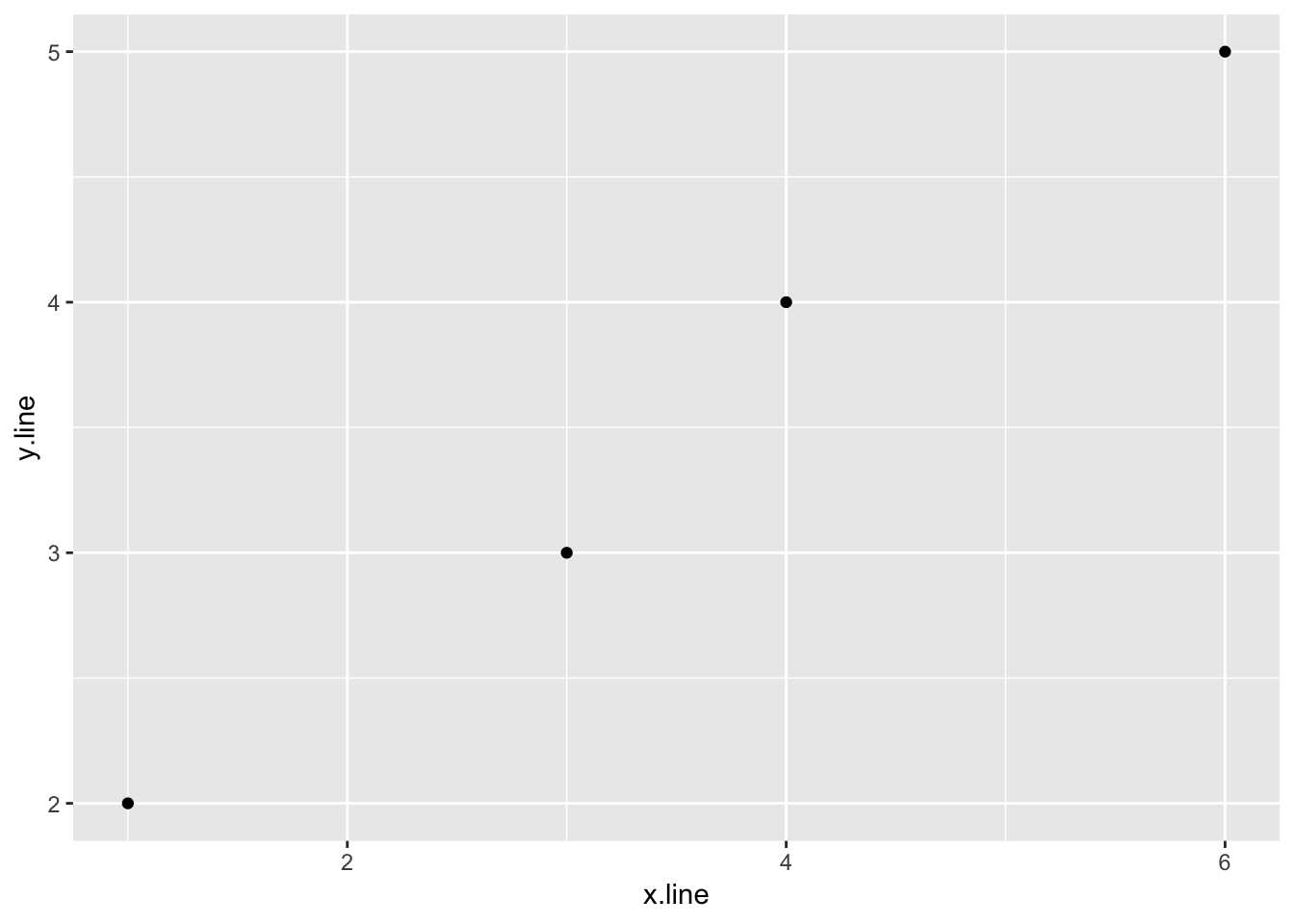
4.2.1.2 Linear regression
Below, the data is fit to the line
\[ y = mx + b \]
the intercept is assumed unless explicity removed using either y ~ x -1 or y ~ 0 + x.
m_sl <- lm(y.line ~ x.line,
          data = simple_line)
m_sl
##
## Call:
## lm(formula = y.line ~ x.line, data = simple_line)
##
## Coefficients:
## (Intercept) x.line
## 1.3462 0.6154summary(m_sl)##
## Call:
## lm(formula = y.line ~ x.line, data = simple_line)
##
## Residuals:
## 1 2 3 4
## 0.03846 -0.19231 0.19231 -0.03846
##
## Coefficients:
## Estimate Std. Error t value Pr(>|t|)
## (Intercept) 1.34615 0.21414 6.286 0.02438 *
## x.line 0.61538 0.05439 11.314 0.00772 **
## ---
## Signif. codes: 0 '***' 0.001 '**' 0.01 '*' 0.05 '.' 0.1 ' ' 1
##
## Residual standard error: 0.1961 on 2 degrees of freedom
## Multiple R-squared: 0.9846, Adjusted R-squared: 0.9769
## F-statistic: 128 on 1 and 2 DF, p-value: 0.007722tidy(m_sl)## # A tibble: 2 x 5
## term estimate std.error statistic p.value
## <chr> <dbl> <dbl> <dbl> <dbl>
## 1 (Intercept) 1.35 0.214 6.29 0.0244
## 2 x.line 0.615 0.0544 11.3 0.00772sl_slope <- tidy(m_sl) %>%
filter(term == "x.line") %>%
dplyr::select(estimate)
sl_intercept <- tidy(m_sl) %>%
filter(term == "(Intercept)") %>%
dplyr::select(estimate)
sl_slope## # A tibble: 1 x 1
## estimate
## <dbl>
## 1 0.615sl_intercept## # A tibble: 1 x 1
## estimate
## <dbl>
## 1 1.354.2.1.3 Plot of the data and linear regression
ggplot(simple_line, aes(x.line, y.line)) +
  geom_point() +
  geom_abline(slope = sl_slope$estimate, intercept = sl_intercept$estimate) +
  ylim(0,6) +
  xlim(0,7)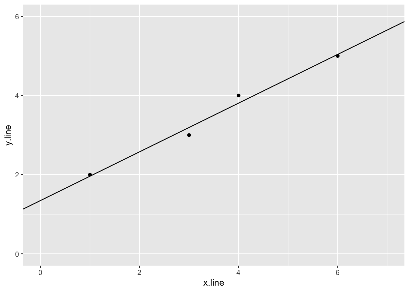
If we don’t need the coeficients, we can plot the data and linear regression using ggplot2
ggplot(simple_line, aes(x.line, y.line)) +
  geom_point() +
  stat_smooth(method = lm, linetype = "dashed") +
  ylim(0,6) +
  xlim(0,7)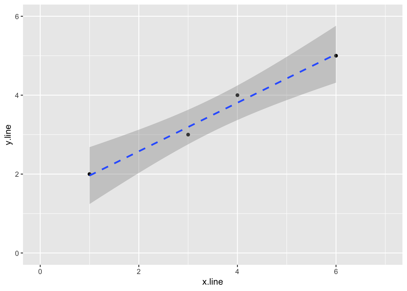
4.2.1.4 Finally, let’s add prediction intervals to the graph
temp_var <- m_sl %>%
  predict(interval="predict") %>%
  as_tibble()
## Warning in predict.lm(., interval = "predict"): predictions on current data refer to _future_ responsestemp_var## # A tibble: 4 x 3
## fit lwr upr
## <dbl> <dbl> <dbl>
## 1 1.96 0.851 3.07
## 2 3.19 2.24 4.14
## 3 3.81 2.86 4.76
## 4 5.04 3.93 6.15simple_line_predict <- bind_cols(simple_line, temp_var)
simple_line_predict## # A tibble: 4 x 5
## x.line y.line fit lwr upr
## <dbl> <dbl> <dbl> <dbl> <dbl>
## 1 1 2 1.96 0.851 3.07
## 2 3 3 3.19 2.24 4.14
## 3 4 4 3.81 2.86 4.76
## 4 6 5 5.04 3.93 6.15ggplot(simple_line_predict, aes(x.line, y.line)) +
geom_point() +
stat_smooth(method = lm, linetype = "dashed", size = 0.5) +
geom_line(aes(y=lwr), color = "red", linetype = "dashed") +
geom_line(aes(y=upr), color = "red", linetype = "dashed") +
ylim(0,7) +
xlim(0,7)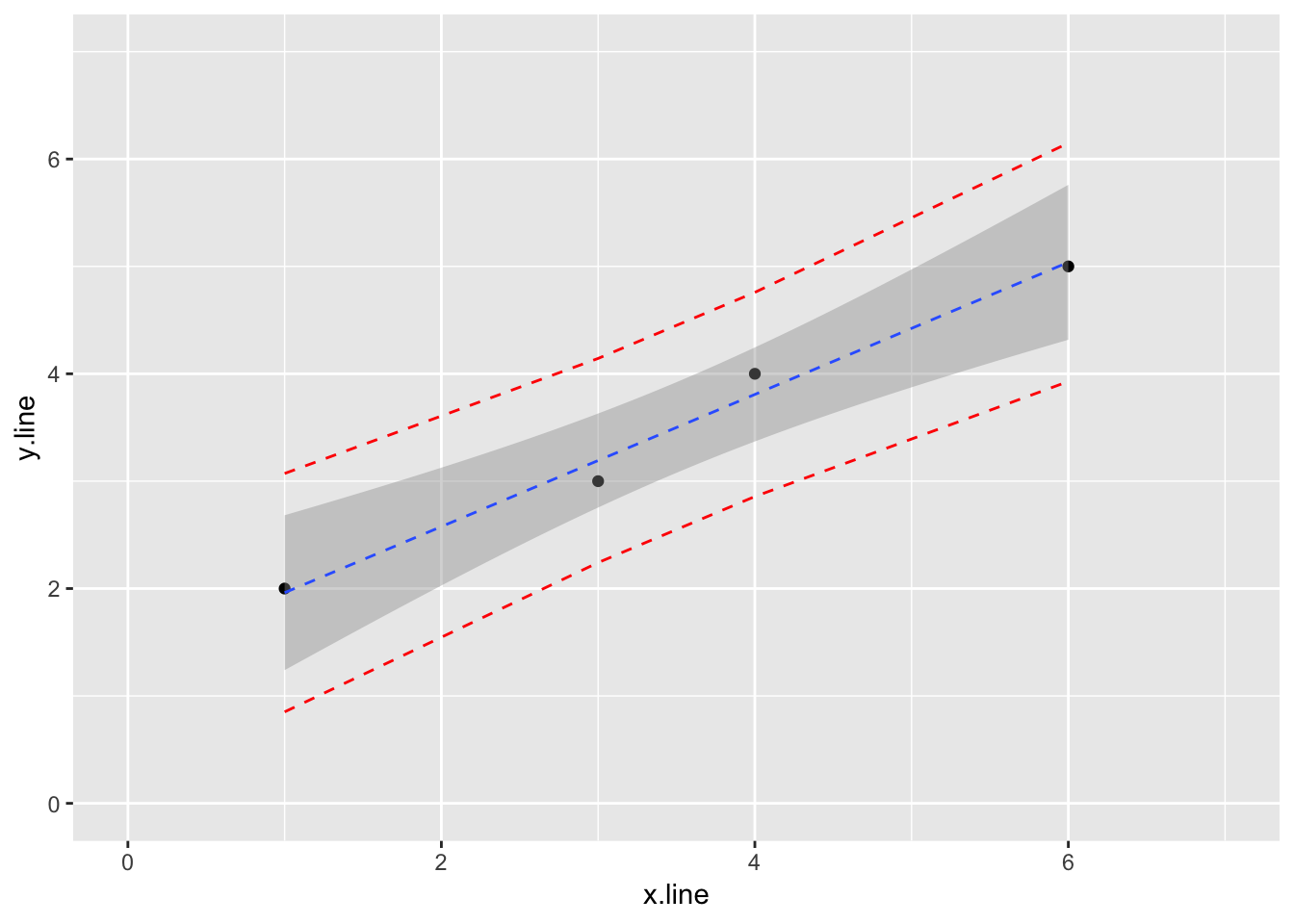
4.2.2 Beyond the linear regression
4.2.2.1 A simple data set for non-linear regression modeling—exponential decay
Example is from Brown, LeMay.
kinetics1 <- tribble(
  ~time, ~conc,
  0., 0.100,
  50., 0.0905,
  100., 0.0820,
  150., 0.0741,
  200., 0.0671,
  300., 0.0549,
  400., 0.0448,
  500., 0.0368,
  800., 0.0200
)
kinetics1
## # A tibble: 9 x 2
## time conc
## <dbl> <dbl>
## 1 0 0.1
## 2 50 0.0905
## 3 100 0.082
## 4 150 0.0741
## 5 200 0.0671
## 6 300 0.0549
## 7 400 0.0448
## 8 500 0.0368
## 9 800 0.024.2.2.2 Simple plots of the data
We can plot the orginal data set, conc vs. time to view the trend. A simple test to confirm the data follows a first-order decay, we can plot log(conc) vs. time.
ggplot(kinetics1, aes(time, conc)) +
  geom_point()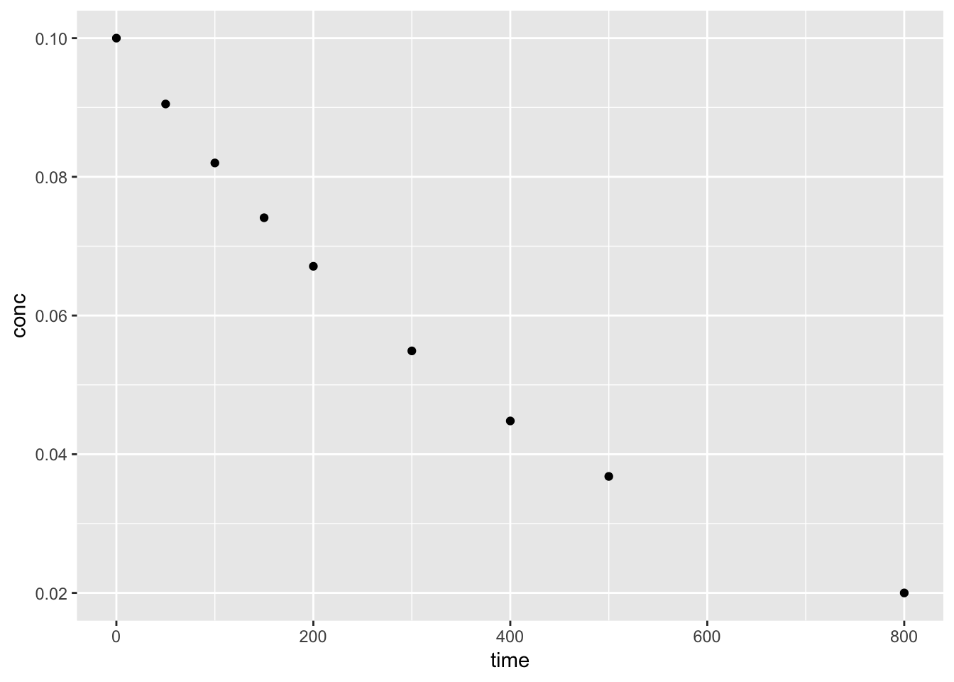
ggplot(kinetics1, aes(time, log(conc))) +
  geom_point()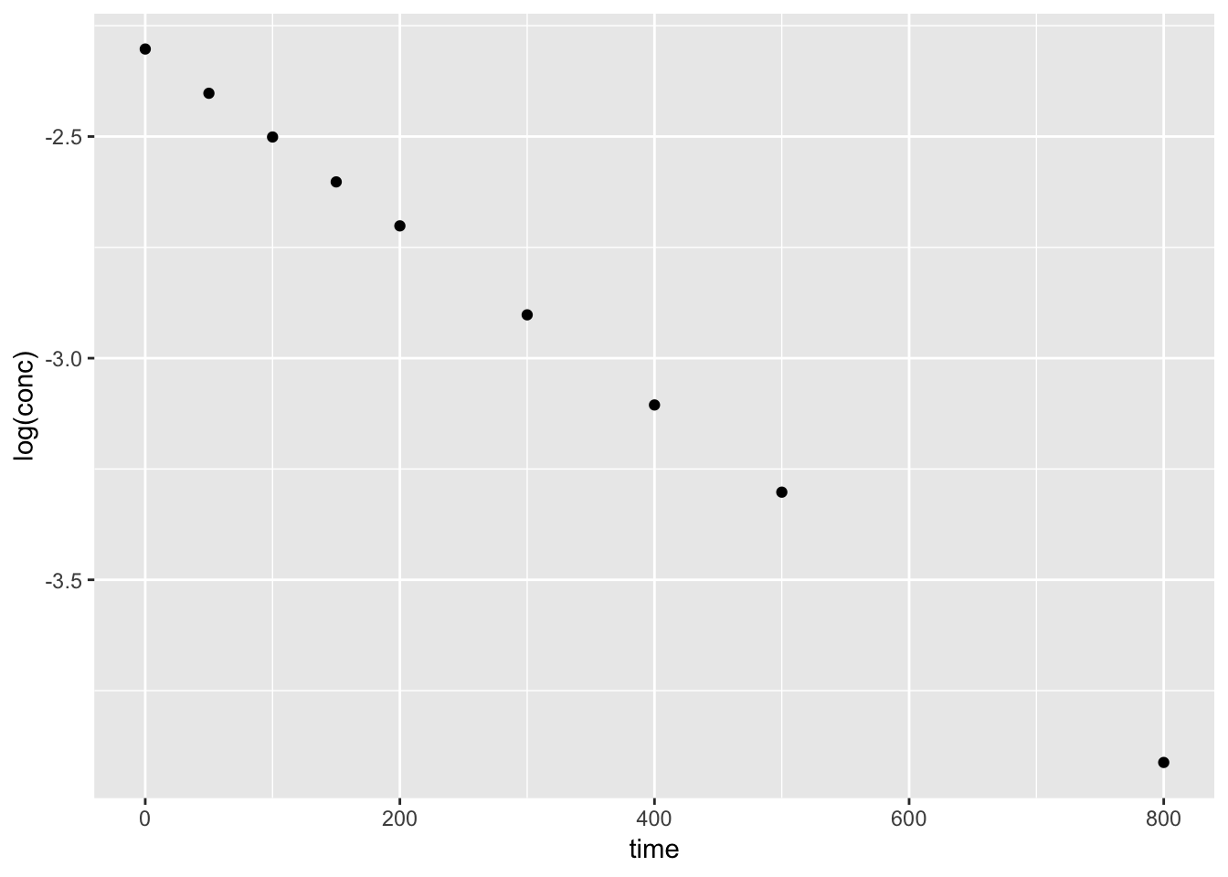
4.2.2.3 Using the nls function
k1 <- nls(conc ~ 0.1*exp(-a1*time),
          data = kinetics1, start = list(a1 = 0.002), trace = T)
## 7.545743e-08 : 0.002
## 7.088224e-08 : 0.0020017
## 7.088224e-08 : 0.002001699summary(k1)##
## Formula: conc ~ 0.1 * exp(-a1 * time)
##
## Parameters:
## Estimate Std. Error t value Pr(>|t|)
## a1 2.002e-03 2.367e-06 845.8 <2e-16 ***
## ---
## Signif. codes: 0 '***' 0.001 '**' 0.01 '*' 0.05 '.' 0.1 ' ' 1
##
## Residual standard error: 9.413e-05 on 8 degrees of freedom
##
## Number of iterations to convergence: 2
## Achieved convergence tolerance: 2.138e-074.2.2.4 Ploting the model results
Using the augment() function from the broom package, we can plot both the data and predicted values from th nls() model.
augment(k1)## # A tibble: 9 x 4
## time conc .fitted .resid
## <dbl> <dbl> <dbl> <dbl>
## 1 0 0.1 0.1 0
## 2 50 0.0905 0.0905 0.0000239
## 3 100 0.082 0.0819 0.000141
## 4 150 0.0741 0.0741 0.0000371
## 5 200 0.0671 0.0670 0.0000908
## 6 300 0.0549 0.0549 0.0000468
## 7 400 0.0448 0.0449 -0.000102
## 8 500 0.0368 0.0368 0.0000433
## 9 800 0.02 0.0202 -0.000162ggplot()+
geom_point(aes(time, conc), kinetics1) +
geom_line(aes(time, .fitted), augment(k1))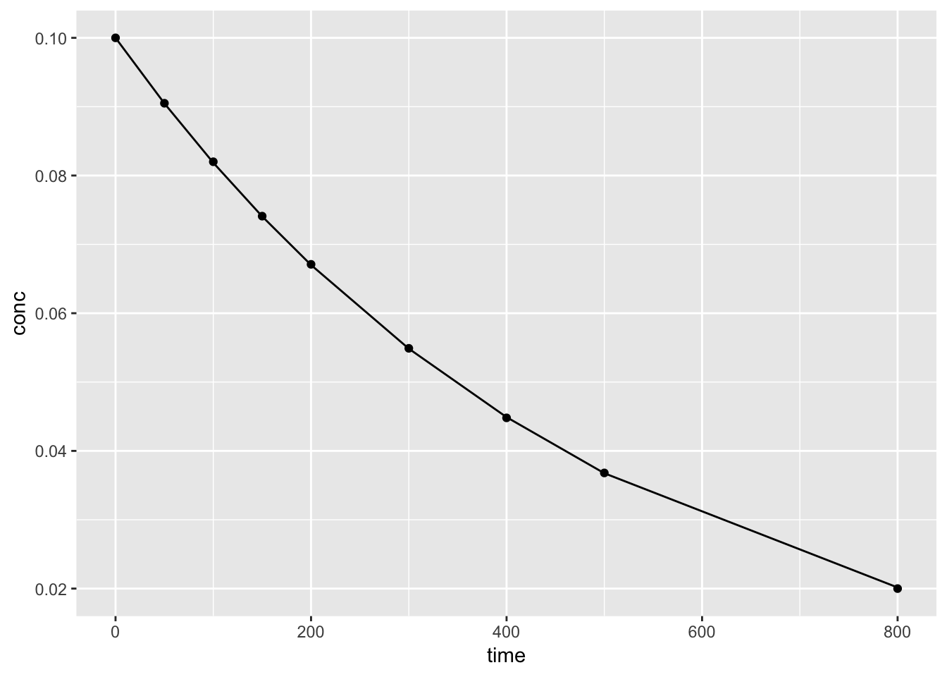
We can also use the output of augment() to plot the residuals
ggplot()+
  geom_point(aes(time, .resid), augment(k1)) +
  geom_hline(yintercept = 0)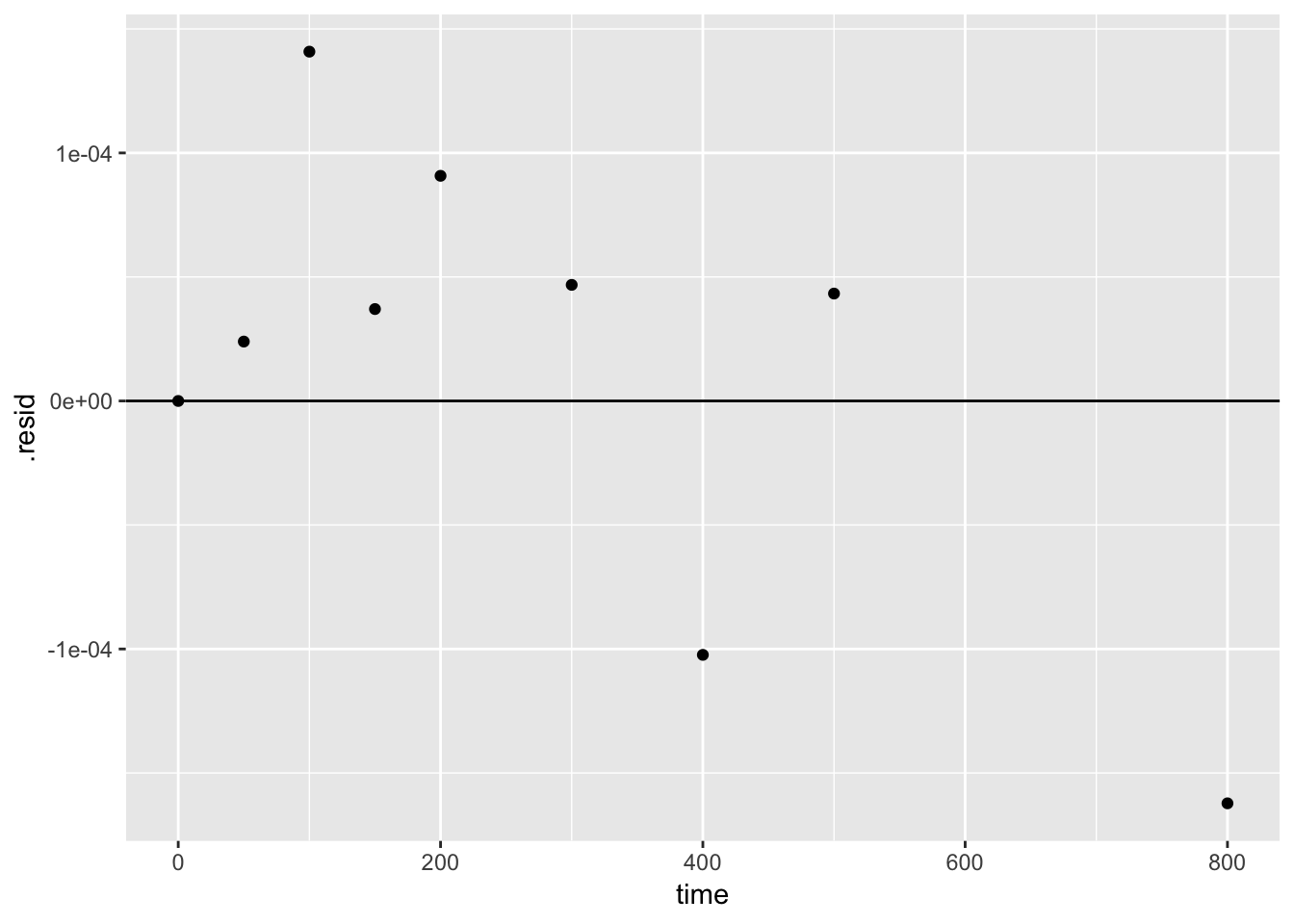
4.2.2.4.1 create a function for the fit
If we want to create a smooth curve of the fit, we need to create a function and use the calculated coefficients from the nls() model. We can then use the stat_function() geom to superimpose the function on the base plot.
conc.fit <- function(t) {
  0.1*exp(-t*summary(k1)$coefficients[1])
  }

ggplot(kinetics1, mapping = aes(time, conc)) +
  geom_point() +
  stat_function(fun = conc.fit, linetype = "dashed", colour = "green") +
  ggtitle("A kinetics example from first-year chemistry", subtitle = "dashed green line: first-order, exponential decay") +
  theme_bw()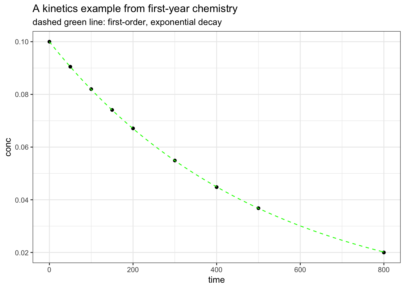
4.3 Case Stuidies
4.3.1 Load cell output
The data collected in the calibration experiment consisted of a known load, applied to the load cell, and the corresponding deflection of the cell from its nominal position. Forty measurements were made over a range of loads from 150,000 to 3,000,000 units. The data were collected in two sets in order of increasing load. The systematic run order makes it difficult to determine whether or not there was any drift in the load cell or measuring equipment over time. Assuming there is no drift, however, the experiment should provide a good description of the relationship between the load applied to the cell and its response.
library(tidyverse)

load_cell <- read_table2(
  "NIST data/PONTIUS.dat", skip = 25, col_names = FALSE, col_types = "dd") %>%
  rename(Deflection = X1, Load = X2)
load_cell
## # A tibble: 40 x 2
## Deflection Load
## <dbl> <dbl>
## 1 0.110 150000
## 2 0.220 300000
## 3 0.329 450000
## 4 0.439 600000
## 5 0.548 750000
## 6 0.657 900000
## 7 0.766 1050000
## 8 0.875 1200000
## 9 0.983 1350000
## 10 1.09 1500000
## # … with 30 more rows4.3.1.1 Selection of Inital Model
First, let’s view the data.
ggplot(load_cell) +
  geom_point(aes(Load, Deflection))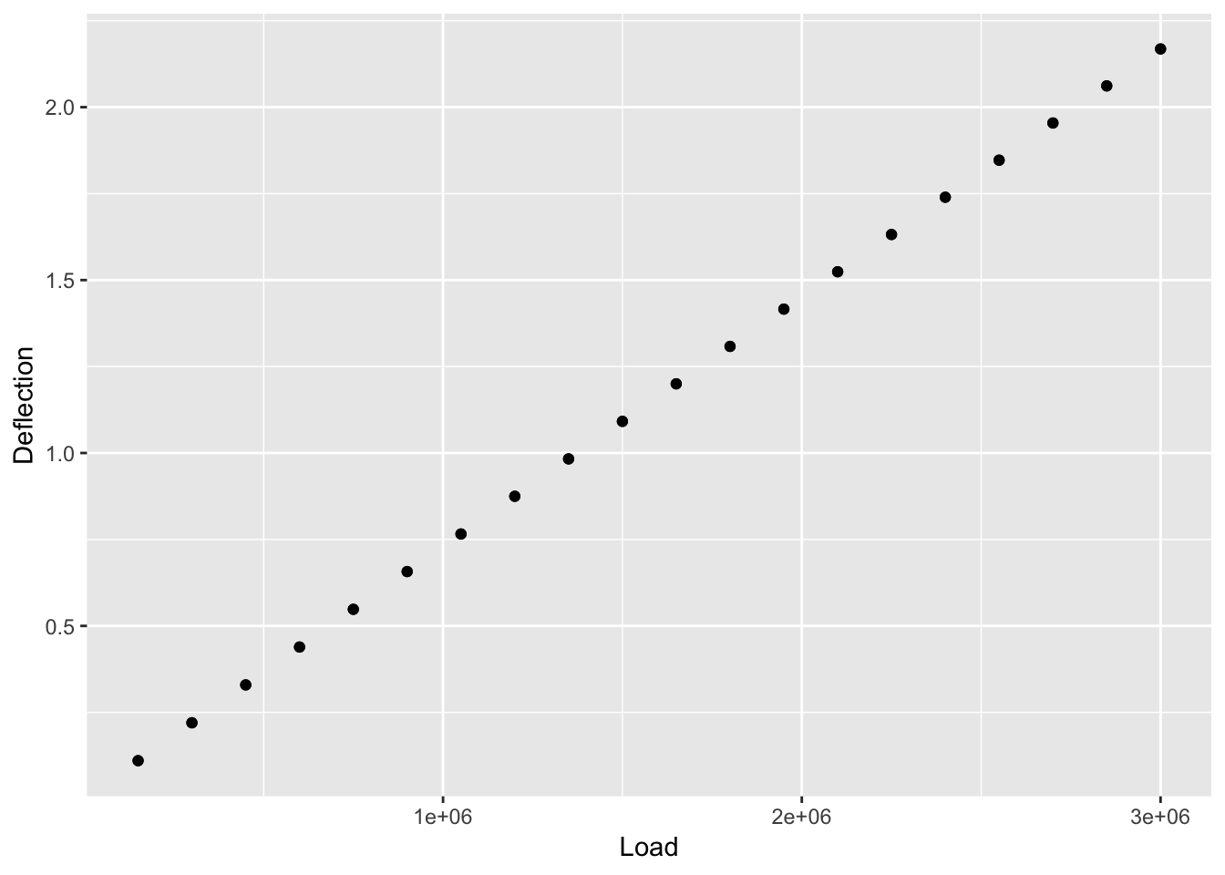
The data looks linear. We can use a simple linear model to view the data
\[ y = mx + b \]
load_cell_model <- lm(Deflection ~ Load, load_cell)
summary(load_cell_model)
##
## Call:
## lm(formula = Deflection ~ Load, data = load_cell)
##
## Residuals:
## Min 1Q Median 3Q Max
## -0.0042751 -0.0016308 0.0005818 0.0018932 0.0024211
##
## Coefficients:
## Estimate Std. Error t value Pr(>|t|)
## (Intercept) 6.150e-03 7.132e-04 8.623 1.77e-10 ***
## Load 7.221e-07 3.969e-10 1819.289 < 2e-16 ***
## ---
## Signif. codes: 0 '***' 0.001 '**' 0.01 '*' 0.05 '.' 0.1 ' ' 1
##
## Residual standard error: 0.002171 on 38 degrees of freedom
## Multiple R-squared: 1, Adjusted R-squared: 1
## F-statistic: 3.31e+06 on 1 and 38 DF, p-value: < 2.2e-16Wow! an R-squared value of 1! it must be perfect.
4.3.1.1.1 A new package to work with summary information: broom()
broom package is part of the tidyverse and inccludes glance(), tidy, and augment().
These functions create tidy data frames based on the model.
load_cell_glance <- glance(load_cell_model)
load_cell_glance
## # A tibble: 1 x 11
## r.squared adj.r.squared sigma statistic p.value df logLik AIC
## <dbl> <dbl> <dbl> <dbl> <dbl> <int> <dbl> <dbl>
## 1 1.000 1.000 0.00217 3309811. 1.77e-95 2 190. -373.
## # … with 3 more variables: BIC <dbl>, deviance <dbl>, df.residual <int>load_cell_tidy <- tidy(load_cell_model)
load_cell_tidy## # A tibble: 2 x 5
## term estimate std.error statistic p.value
## <chr> <dbl> <dbl> <dbl> <dbl>
## 1 (Intercept) 0.00615 7.13e- 4 8.62 1.77e-10
## 2 Load 0.000000722 3.97e-10 1819. 1.77e-95augment(load_cell_model)## # A tibble: 40 x 9
## Deflection Load .fitted .se.fit .resid .hat .sigma .cooksd
## <dbl> <dbl> <dbl> <dbl> <dbl> <dbl> <dbl> <dbl>
## 1 0.110 1.50e5 0.114 6.62e-4 -4.28e-3 0.0929 0.00207 2.19e-1
## 2 0.220 3.00e5 0.223 6.12e-4 -3.22e-3 0.0793 0.00213 1.03e-1
## 3 0.329 4.50e5 0.331 5.63e-4 -1.61e-3 0.0673 0.00218 2.12e-2
## 4 0.439 6.00e5 0.439 5.17e-4 -4.21e-4 0.0568 0.00220 1.20e-3
## 5 0.548 7.50e5 0.548 4.74e-4 3.03e-4 0.0477 0.00220 5.14e-4
## 6 0.657 9.00e5 0.656 4.35e-4 8.98e-4 0.0402 0.00220 3.73e-3
## 7 0.766 1.05e6 0.764 4.02e-4 1.26e-3 0.0342 0.00219 6.20e-3
## 8 0.875 1.20e6 0.873 3.74e-4 2.20e-3 0.0297 0.00217 1.62e-2
## 9 0.983 1.35e6 0.981 3.55e-4 1.93e-3 0.0267 0.00218 1.12e-2
## 10 1.09 1.50e6 1.09 3.45e-4 2.16e-3 0.0252 0.00217 1.31e-2
## # … with 30 more rows, and 1 more variable: .std.resid <dbl>ggplot(load_cell, aes(Load, Deflection)) +
geom_point() +
stat_smooth(method = lm, linetype = "dashed", colour = "blue", size = 0.5) +
ggtitle("NIST Load Cell Calibration Data", subtitle = "+/- 95% Confidence Intervals are not visible")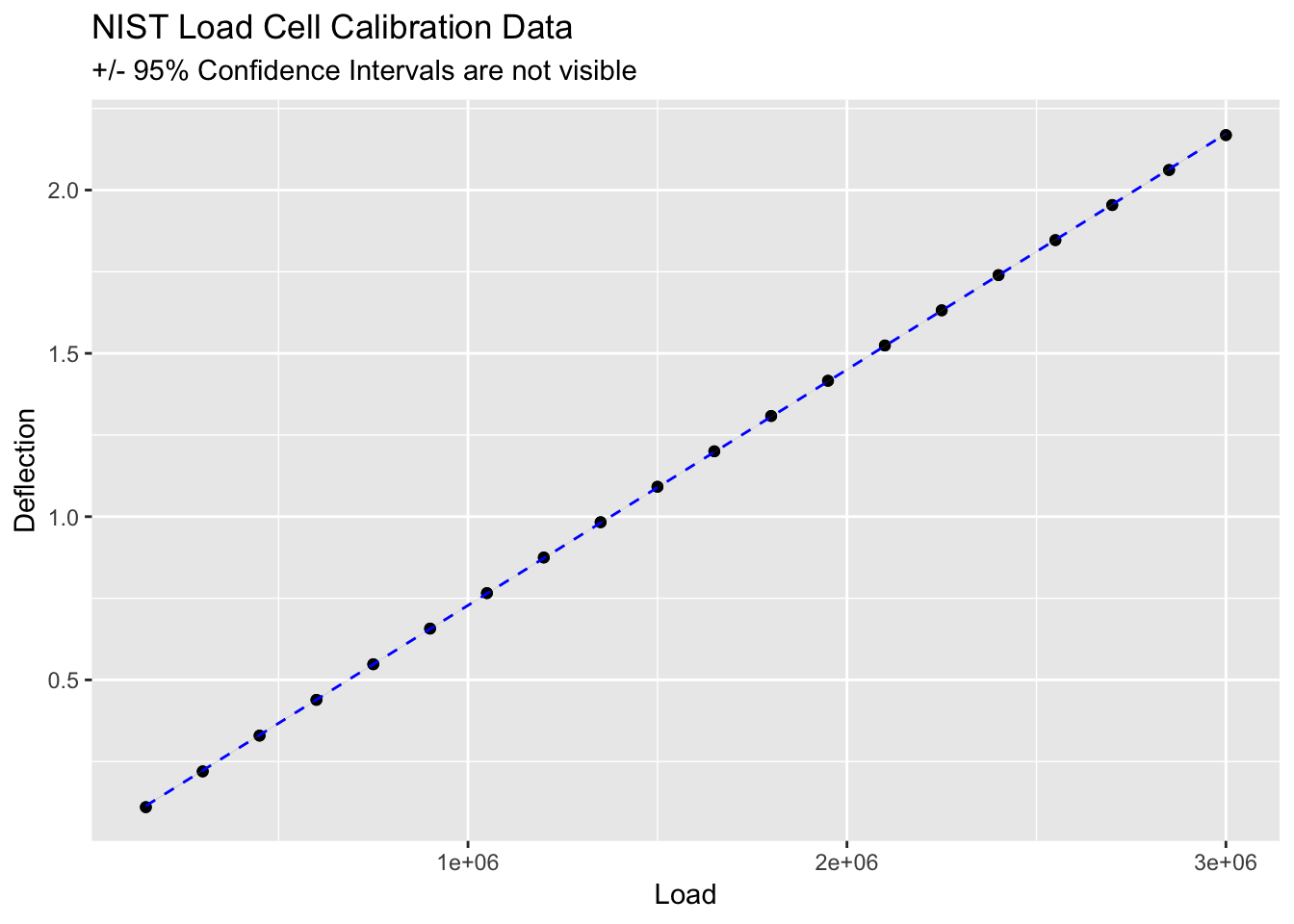
4.3.1.2 But wait! What about the residuals?
load_cell_resid = resid(load_cell_model)
load_cell_resid
## 1 2 3 4 5
## -0.0042750714 -0.0032204586 -0.0016058459 -0.0004212331 0.0003033797
## 6 7 8 9 10
## 0.0008979925 0.0012626053 0.0021972180 0.0019318308 0.0021564436
## 11 12 13 14 15
## 0.0023910564 0.0022856692 0.0017402820 0.0014248947 0.0010595075
## 16 17 18 19 20
## 0.0002741203 -0.0010512669 -0.0019066541 -0.0028620414 -0.0040174286
## 21 22 23 24 25
## -0.0039450714 -0.0026004586 -0.0017058459 -0.0005512331 0.0002533797
## 26 27 28 29 30
## 0.0013479925 0.0016026053 0.0020672180 0.0020118308 0.0021964436
## 31 32 33 34 35
## 0.0024210564 0.0022456692 0.0018802820 0.0015148947 0.0007095075
## 36 37 38 39 40
## 0.0004541203 -0.0005512669 -0.0013766541 -0.0023720414 -0.0041674286# ggplot() +
# geom_point(aes(LoadCell$Load, LC.resid)) +
# geom_hline(aes(yintercept=0)) +
# geom_hline(aes(yintercept=+2*(summary(m.LC)$sigma)), linetype = "dashed") +
# geom_hline(aes(yintercept=-2*(summary(m.LC)$sigma)), linetype = "dashed") +
# ggtitle("Deflection Load Residuals", subtitle = "+/- 2(Residual Statndard Deviation)") +
# theme(plot.title = element_text(hjust = 0.5), plot.subtitle = element_text(hjust = 0.5))Using the augment() function we can plot the residuals very easily
load_cell_fit <- augment(load_cell_model)
load_cell_fit
## # A tibble: 40 x 9
## Deflection Load .fitted .se.fit .resid .hat .sigma .cooksd
## <dbl> <dbl> <dbl> <dbl> <dbl> <dbl> <dbl> <dbl>
## 1 0.110 1.50e5 0.114 6.62e-4 -4.28e-3 0.0929 0.00207 2.19e-1
## 2 0.220 3.00e5 0.223 6.12e-4 -3.22e-3 0.0793 0.00213 1.03e-1
## 3 0.329 4.50e5 0.331 5.63e-4 -1.61e-3 0.0673 0.00218 2.12e-2
## 4 0.439 6.00e5 0.439 5.17e-4 -4.21e-4 0.0568 0.00220 1.20e-3
## 5 0.548 7.50e5 0.548 4.74e-4 3.03e-4 0.0477 0.00220 5.14e-4
## 6 0.657 9.00e5 0.656 4.35e-4 8.98e-4 0.0402 0.00220 3.73e-3
## 7 0.766 1.05e6 0.764 4.02e-4 1.26e-3 0.0342 0.00219 6.20e-3
## 8 0.875 1.20e6 0.873 3.74e-4 2.20e-3 0.0297 0.00217 1.62e-2
## 9 0.983 1.35e6 0.981 3.55e-4 1.93e-3 0.0267 0.00218 1.12e-2
## 10 1.09 1.50e6 1.09 3.45e-4 2.16e-3 0.0252 0.00217 1.31e-2
## # … with 30 more rows, and 1 more variable: .std.resid <dbl>ggplot(load_cell_fit) +
geom_point(aes(Load, .resid)) +
ggtitle("Residuals from linear model of the load cell")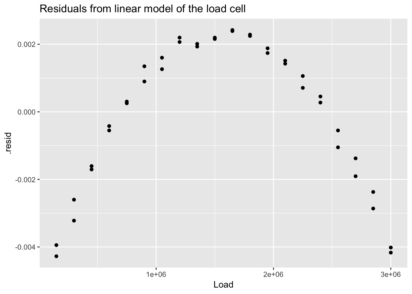
The residuals from a good model would be random. Although not necessary, we can plot a histogram or qqplot to demonstrate the residuals are not following a normal distribution.
ggplot(load_cell_fit) +
  geom_histogram(aes(.resid))
## `stat_bin()` using `bins = 30`. Pick better value with `binwidth`.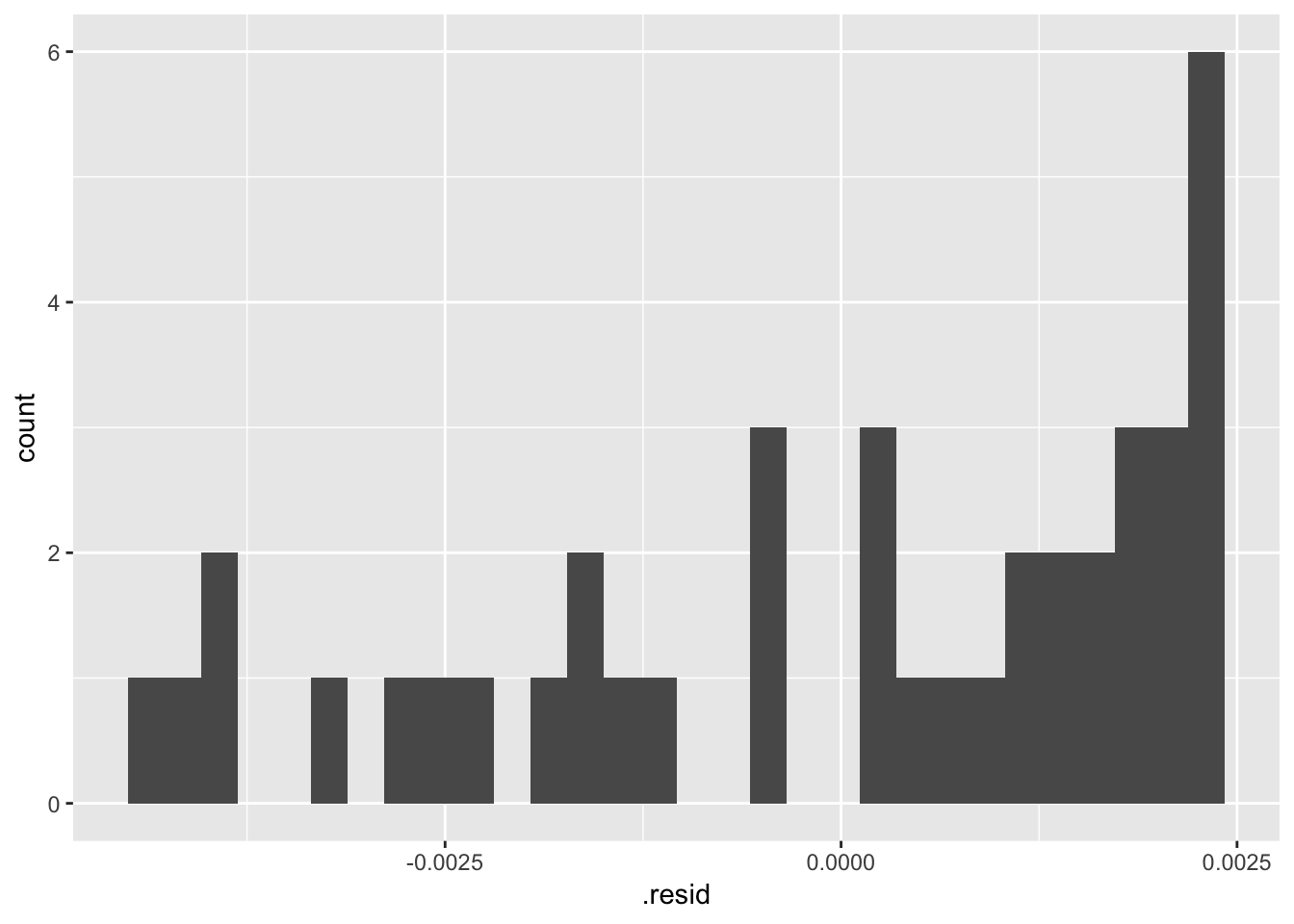
ggplot(load_cell_fit) +
  geom_qq(aes(sample = .resid))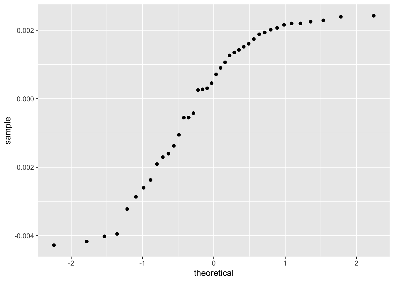
4.3.1.3 Model Refinement
\[ D = \beta_0 + \beta_1 L + \beta_2 L^2 + \varepsilon \]
We can use the linear model function, lm(), by creating a new variable \(L^2\).
load_cell_2 <- mutate(load_cell, Load_squared = Load^2)
load_cell_2
## # A tibble: 40 x 3
## Deflection Load Load_squared
## <dbl> <dbl> <dbl>
## 1 0.110 150000 22500000000
## 2 0.220 300000 90000000000
## 3 0.329 450000 202500000000
## 4 0.439 600000 360000000000
## 5 0.548 750000 562500000000
## 6 0.657 900000 810000000000
## 7 0.766 1050000 1102500000000
## 8 0.875 1200000 1440000000000
## 9 0.983 1350000 1822500000000
## 10 1.09 1500000 2250000000000
## # … with 30 more rowsload_cell_model_2 <- lm(Deflection ~ Load + Load_squared, load_cell_2)
summary(load_cell_model_2)##
## Call:
## lm(formula = Deflection ~ Load + Load_squared, data = load_cell_2)
##
## Residuals:
## Min 1Q Median 3Q Max
## -4.468e-04 -1.578e-04 3.817e-05 1.088e-04 4.235e-04
##
## Coefficients:
## Estimate Std. Error t value Pr(>|t|)
## (Intercept) 6.736e-04 1.079e-04 6.24 2.97e-07 ***
## Load 7.321e-07 1.578e-10 4638.65 < 2e-16 ***
## Load_squared -3.161e-15 4.867e-17 -64.95 < 2e-16 ***
## ---
## Signif. codes: 0 '***' 0.001 '**' 0.01 '*' 0.05 '.' 0.1 ' ' 1
##
## Residual standard error: 0.0002052 on 37 degrees of freedom
## Multiple R-squared: 1, Adjusted R-squared: 1
## F-statistic: 1.853e+08 on 2 and 37 DF, p-value: < 2.2e-16load_cell_fit_2 <- augment(load_cell_model_2)
load_cell_fit_2## # A tibble: 40 x 10
## Deflection Load Load_squared .fitted .se.fit .resid .hat .sigma
## <dbl> <dbl> <dbl> <dbl> <dbl> <dbl> <dbl> <dbl>
## 1 0.110 1.50e5 2.25e10 0.110 8.83e-5 -2.21e-4 0.185 2.04e-4
## 2 0.220 3.00e5 9.00e10 0.220 7.19e-5 -4.47e-4 0.123 1.92e-4
## 3 0.329 4.50e5 2.02e11 0.329 5.89e-5 2.99e-5 0.0824 2.08e-4
## 4 0.439 6.00e5 3.60e11 0.439 4.99e-5 2.19e-4 0.0591 2.05e-4
## 5 0.548 7.50e5 5.62e11 0.548 4.50e-5 9.00e-5 0.0480 2.07e-4
## 6 0.657 9.00e5 8.10e11 0.657 4.35e-5 -2.65e-5 0.0450 2.08e-4
## 7 0.766 1.05e6 1.10e12 0.766 4.44e-5 -2.31e-4 0.0468 2.04e-4
## 8 0.875 1.20e6 1.44e12 0.875 4.61e-5 2.77e-4 0.0505 2.03e-4
## 9 0.983 1.35e6 1.82e12 0.983 4.77e-5 -2.73e-4 0.0541 2.03e-4
## 10 1.09 1.50e6 2.25e12 1.09 4.86e-5 -1.90e-4 0.0562 2.05e-4
## # … with 30 more rows, and 2 more variables: .cooksd <dbl>,
## # .std.resid <dbl>ggplot(load_cell_fit_2) +
geom_point(aes(Load, .resid)) +
ggtitle("Residuals from refined model of the load cell")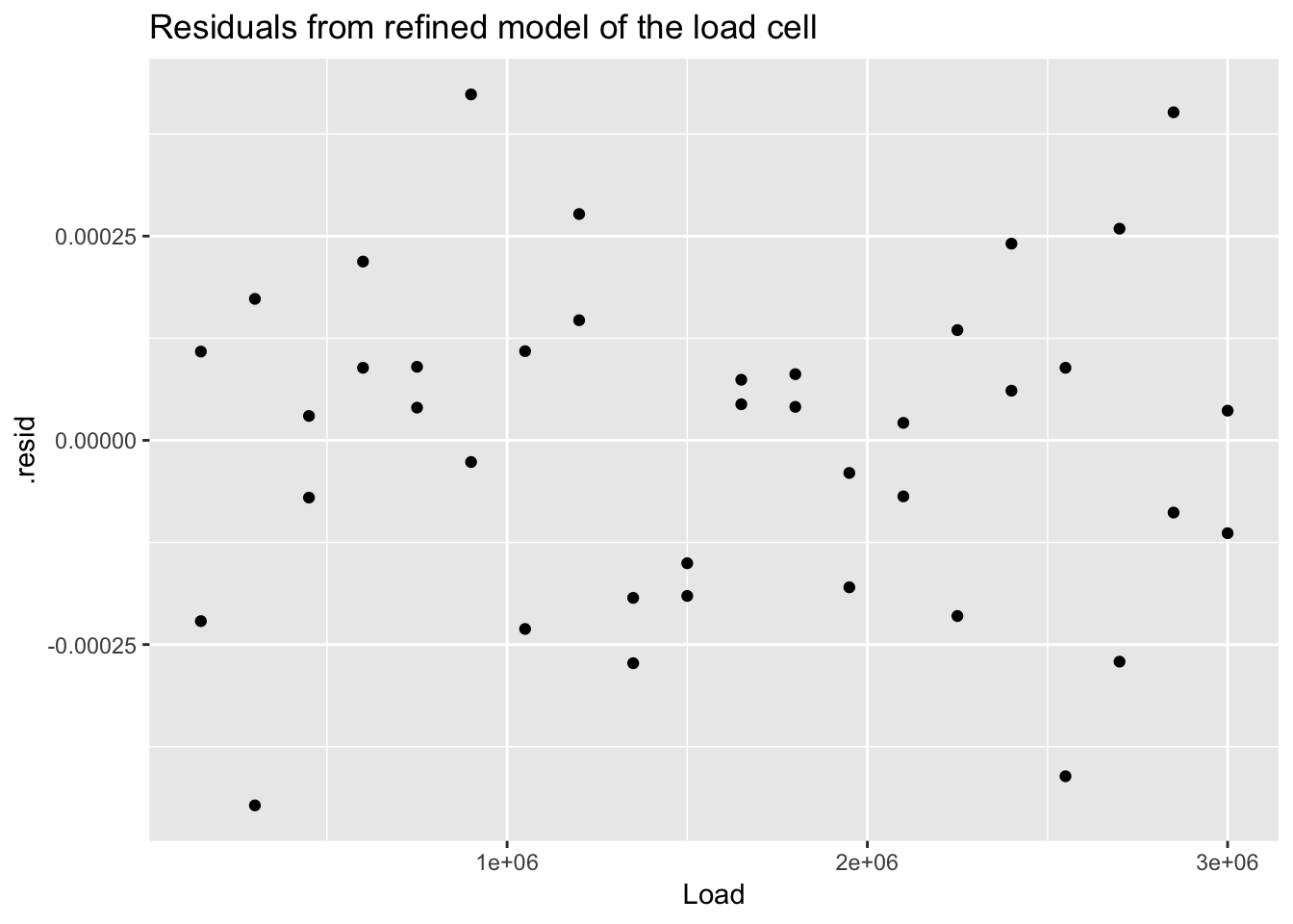
4.3.1.3.1 Could we have used a non-linear least squares fit model?
load_cell_model_3 <- nls(Deflection ~ b0 + b1*Load + b2*Load^2, load_cell_2, start = c(b0 = 0, b1 = 0,b2 = 0))

summary(load_cell_model_3)
##
## Formula: Deflection ~ b0 + b1 * Load + b2 * Load^2
##
## Parameters:
## Estimate Std. Error t value Pr(>|t|)
## b0 6.736e-04 1.079e-04 6.24 2.97e-07 ***
## b1 7.321e-07 1.578e-10 4638.65 < 2e-16 ***
## b2 -3.161e-15 4.867e-17 -64.95 < 2e-16 ***
## ---
## Signif. codes: 0 '***' 0.001 '**' 0.01 '*' 0.05 '.' 0.1 ' ' 1
##
## Residual standard error: 0.0002052 on 37 degrees of freedom
##
## Number of iterations to convergence: 1
## Achieved convergence tolerance: 1.328e-06The results are identical.
ggplot(load_cell_fit_2) +
  geom_histogram(aes(.resid))
## `stat_bin()` using `bins = 30`. Pick better value with `binwidth`.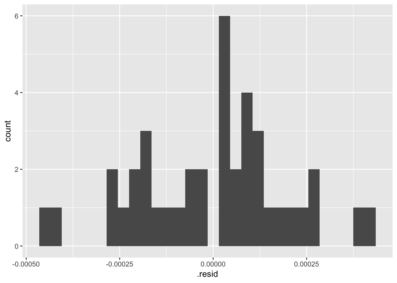
ggplot(load_cell_fit_2) +
  geom_qq(aes(sample = .resid))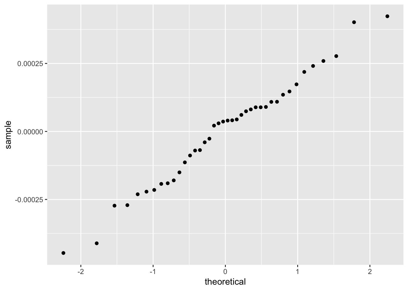
4.3.2 Thermal expansion of copper
from section 4.6.4. Thermal Expansion of Copper Case Study
This case study illustrates the use of a class of nonlinear models called rational function models. The data set used is the thermal expansion of copper related to temperature.
CTECu <- read_table2(
  "NIST data/HAHN1.dat", skip = 25, col_names = FALSE)
## Parsed with column specification:
## cols(
## X1 = col_double(),
## X2 = col_double()
## )CTECu <- CTECu %>%
rename(temp_K = X1, Cu_CTE = X2)
View(CTECu)ggplot(CTECu, aes(temp_K, Cu_CTE)) +
geom_point()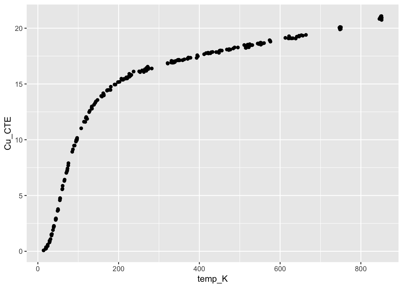
4.3.3 Quadratic/Quadratic (Q/Q) model
The NIST handbook has a procedure for calculing estimates for the model, below, I just used guess values for the equation \[ y = \frac{(A0 + A1 \cdot x + A2 \cdot x^2)}{(1 + B1\cdot x + B2 \cdot X^2)} \]
model_Cu <- nls(Cu_CTE ~ ((a0 + a1*temp_K + a2*temp_K^2)/(1 + b1*temp_K + b2*temp_K^2)),
CTECu, start = list(a0 = 0, a1 = -1, a2 = -1, b1 = 0, b2 = 0), trace = T)## 1.344556e+13 : 0 -1 -1 0 0
## 1697329 : -3.351400e+00 1.797879e-01 -5.745645e-04 7.915158e-07 -3.877688e-10
## 177589.3 : -3.319661e+00 1.750319e-01 -3.592189e-04 1.144561e-03 -6.445222e-07
## 32411.82 : -4.730736e+00 2.146213e-01 -3.235814e-04 3.851759e-03 -2.232626e-06
## 5374.946 : -6.413603e+00 2.683958e-01 -2.844465e-04 7.799104e-03 -4.266107e-06
## 690.5713 : -6.901674e+00 2.867489e-01 -1.804611e-04 1.009256e-02 -3.131612e-06
## 217.1164 : -5.970973e+00 2.481232e-01 1.250216e-04 8.918691e-03 1.150181e-05
## 114.0929 : -3.145220e+00 1.061122e-01 1.610442e-03 4.783451e-03 8.707152e-05
## 64.59622 : 3.1477349163 -0.2965983768 0.0078946767 0.0013004690 0.0003974542
## 42.78158 : 9.3230025114 -0.8210512798 0.0188009501 0.0103976361 0.0009147904
## 34.34313 : 11.848742450 -1.098105431 0.025888747 0.024139632 0.001231568
## 33.5614 : 11.838847499 -1.129134608 0.027249383 0.029538247 0.001286009
## 33.55298 : 12.220405792 -1.169396827 0.028259353 0.031296606 0.001332281
## 33.55278 : 11.988150281 -1.149285630 0.027831681 0.030880324 0.001312172
## 33.55273 : 12.165006923 -1.165285413 0.028186412 0.031296535 0.001328754
## 33.55271 : 12.034452089 -1.153533233 0.027926998 0.030997296 0.001316621
## 33.55269 : 12.131480095 -1.162274660 0.028120094 0.031220657 0.001325652
## 33.55268 : 12.059618930 -1.155801947 0.027977138 0.031055397 0.001318966
## 33.55268 : 12.112946981 -1.160605895 0.028083247 0.031178098 0.001323928
## 33.55268 : 12.073406215 -1.157044238 0.028004583 0.031087151 0.001320249
## 33.55267 : 12.102793316 -1.159691514 0.028063056 0.031154770 0.001322984
## 33.55267 : 12.081046435 -1.157732650 0.028019791 0.031104752 0.001320961
## 33.55267 : 12.097167203 -1.159184809 0.028051866 0.031141839 0.001322461
## 33.55267 : 12.085177311 -1.158104731 0.028028009 0.031114250 0.001321345
## 33.55267 : 12.094068505 -1.158905649 0.028045699 0.031134704 0.001322172
## 33.55267 : 12.087436601 -1.158308224 0.028032503 0.031119442 0.001321555
## 33.55267 : 12.092386536 -1.158754113 0.028042351 0.031130832 0.001322016
## 33.55267 : 12.088732963 -1.158425030 0.028035083 0.031122431 0.001321676
## 33.55267 : 12.091445289 -1.158669369 0.028040481 0.031128672 0.001321928
## 33.55267 : 12.08942043 -1.15848695 0.02803645 0.03112401 0.00132174
## 33.55267 : 12.090900623 -1.158620261 0.028039395 0.031127413 0.001321877
## 33.55267 : 12.089833503 -1.158524186 0.028037274 0.031124964 0.001321778
## 33.55267 : 12.090620445 -1.158595059 0.028038839 0.031126773 0.001321851summary(model_Cu)##
## Formula: Cu_CTE ~ ((a0 + a1 * temp_K + a2 * temp_K^2)/(1 + b1 * temp_K +
## b2 * temp_K^2))
##
## Parameters:
## Estimate Std. Error t value Pr(>|t|)
## a0 12.0906204 4.9457268 2.445 0.01525 *
## a1 -1.1585951 0.4459281 -2.598 0.00997 **
## a2 0.0280388 0.0099339 2.823 0.00518 **
## b1 0.0311268 0.0123461 2.521 0.01237 *
## b2 0.0013219 0.0004639 2.849 0.00478 **
## ---
## Signif. codes: 0 '***' 0.001 '**' 0.01 '*' 0.05 '.' 0.1 ' ' 1
##
## Residual standard error: 0.3811 on 231 degrees of freedom
##
## Number of iterations to convergence: 32
## Achieved convergence tolerance: 8.018e-06glance(model_Cu)## # A tibble: 1 x 8
## sigma isConv finTol logLik AIC BIC deviance df.residual
## <dbl> <lgl> <dbl> <dbl> <dbl> <dbl> <dbl> <int>
## 1 0.381 TRUE 0.00000802 -105. 221. 242. 33.6 231augment(model_Cu)## # A tibble: 236 x 4
## temp_K Cu_CTE .fitted .resid
## <dbl> <dbl> <dbl> <dbl>
## 1 24.4 0.591 0.203 0.388
## 2 34.8 1.55 1.56 -0.0110
## 3 44.1 2.90 3.14 -0.237
## 4 45.1 2.89 3.31 -0.413
## 5 55.0 4.70 4.94 -0.239
## 6 65.5 6.31 6.49 -0.181
## 7 70.5 7.03 7.15 -0.119
## 8 75.7 7.90 7.78 0.116
## 9 89.6 9.47 9.26 0.211
## 10 91.1 9.48 9.41 0.0757
## # … with 226 more rowstidy(model_Cu)## # A tibble: 5 x 5
## term estimate std.error statistic p.value
## <chr> <dbl> <dbl> <dbl> <dbl>
## 1 a0 12.1 4.95 2.44 0.0152
## 2 a1 -1.16 0.446 -2.60 0.00997
## 3 a2 0.0280 0.00993 2.82 0.00518
## 4 b1 0.0311 0.0123 2.52 0.0124
## 5 b2 0.00132 0.000464 2.85 0.004784.3.3.1 Create a function using the fit paramters
Cu_fit <- function(x) {
((summary(model_Cu)$coefficients[1] + summary(model_Cu)$coefficients[2]*x + summary(model_Cu)$coefficients[3]*x^2)/(1 + summary(model_Cu)$coefficients[4]*x + summary(model_Cu)$coefficients[5]*x^2))
}4.3.3.2 Add the fitted curve to the graph
ggplot(CTECu, aes(temp_K, Cu_CTE)) +
geom_point() +
stat_function(fun = Cu_fit, colour = "green", linetype = "dashed") +
ggtitle("Thermal Expansion of Copper", subtitle = "nls function using Q/Q model")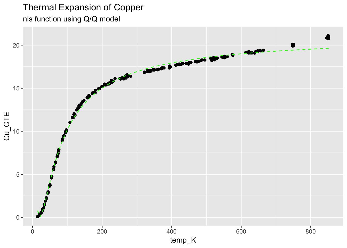
4.3.3.3 Plot the residulas
ggplot(augment(model_Cu)) +
  geom_point(aes(temp_K, .resid)) +
  geom_hline(aes(yintercept=0)) +
  geom_hline(aes(yintercept=+2*(0.38)), linetype = "dashed") +
  geom_hline(aes(yintercept=-2*(0.38)), linetype = "dashed") +
  ggtitle("Thermal Expansion of Copper Residuals", subtitle = "+/- 2(Residual Statndard Deviation)")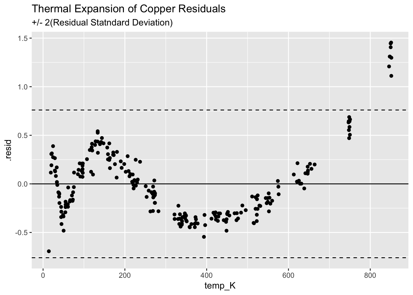
The fit is not very good, shows a clear structure, and indicates the Q/Q model is insufficient.
4.3.4 Cubic/Cubic Rational Function
\[ y = \frac{(A0 + A1*x + A2x^2 + A3X^3)} {(1 + B1x + B2X^2 + B3X^3)} \]
mcc_Cu <- nls(Cu_CTE ~ ((a0 + a1*temp_K + a2*temp_K^2 + a3*temp_K^3)/(1 + b1*temp_K + b2*temp_K^2 + b3*temp_K^3)),
            CTECu, start = list(a0 = 0, a1 = -1, a2 = -1, a3 = 0, b1 = 0, b2 = 0, b3 = 0),
            trace = T)
## 1.344556e+13 : 0 -1 -1 0 0 0 0
## 1.339595e+13 : -4.089856e-03 -9.988271e-01 -9.983564e-01 6.676610e-04 -6.676602e-04 -1.055201e-11 1.803518e-15
## 1.334366e+13 : -4.807459e-03 -9.966232e-01 -9.964072e-01 6.664584e-04 -6.677607e-04 -1.094787e-11 1.584238e-15
## 1.32396e+13 : -6.863478e-03 -9.922082e-01 -9.925166e-01 6.639777e-04 -6.678813e-04 -1.223912e-11 1.510447e-15
## 1.30334e+13 : -1.594000e-02 -9.833127e-01 -9.847661e-01 6.593020e-04 -6.683904e-04 -1.602231e-11 1.289942e-15
## 1.262831e+13 : -6.540076e-02 -9.650849e-01 -9.693885e-01 6.507887e-04 -6.701861e-04 -3.033631e-11 1.802077e-15
## 1.184743e+13 : -1.788916e-01 -9.289031e-01 -9.391153e-01 6.341455e-04 -6.739522e-04 -6.184747e-11 2.875150e-15
## 1.040295e+13 : -4.142861e-01 -8.583930e-01 -8.804668e-01 5.994049e-04 -6.790616e-04 -1.428677e-10 1.605646e-14
## 7.989692e+12 : -9.341122e-01 -7.234575e-01 -7.705432e-01 5.175015e-04 -6.708211e-04 -4.851866e-10 1.813912e-13
## 6.371193e+12 : -1.922326e+00 -4.855256e-01 -5.789681e-01 -4.405781e-04 4.048477e-04 -1.132038e-09 4.421753e-13
## 1.590227e+12 : -3.385858e+00 -1.294959e-01 -2.899297e-01 -2.187966e-04 4.037949e-04 -2.100189e-09 8.979057e-13
## 19889209 : -4.850624e+00 2.266128e-01 -8.927502e-04 3.128700e-06 3.991144e-04 -5.877643e-09 2.695245e-12
## 825292.5 : -4.854099e+00 2.244501e-01 -7.872443e-04 1.327192e-06 8.773391e-04 4.504172e-08 -1.183450e-10
## 72834.96 : -4.698904e+00 2.158071e-01 -6.255161e-04 8.206990e-07 1.206312e-03 1.711327e-06 -1.281084e-09
## 11897.69 : -4.260919e+00 1.962288e-01 -4.518142e-04 6.174559e-07 5.394675e-04 9.144746e-06 -6.252643e-09
## 3068.102 : -3.363680e+00 1.545785e-01 -1.051538e-04 4.250646e-07 -1.433242e-03 2.984461e-05 -2.070801e-08
## 909.5887 : -1.947093e+00 8.097392e-02 6.980495e-04 -2.856405e-08 -4.239912e-03 7.556907e-05 -5.390319e-08
## 220.8618 : -4.057550e-01 -1.376339e-02 2.096694e-03 -9.279485e-07 -6.080614e-03 1.470438e-04 -1.056115e-07
## 31.88262 : 7.090768e-01 -9.381732e-02 3.536101e-03 -1.838264e-06 -6.162496e-03 2.145881e-04 -1.480838e-07
## 3.200182 : 1.102048e+00 -1.249213e-01 4.149347e-03 -1.951524e-06 -5.756966e-03 2.422411e-04 -1.492413e-07
## 1.55733 : 1.100520e+00 -1.246480e-01 4.131519e-03 -1.571143e-06 -5.729023e-03 2.422069e-04 -1.300201e-07
## 1.532465 : 1.080053e+00 -1.228904e-01 4.090638e-03 -1.435504e-06 -5.758189e-03 2.407076e-04 -1.235758e-07
## 1.532438 : 1.077745e+00 -1.227015e-01 4.086549e-03 -1.426532e-06 -5.760914e-03 2.405448e-04 -1.231569e-07
## 1.532438 : 1.077639e+00 -1.226932e-01 4.086381e-03 -1.426274e-06 -5.760992e-03 2.405376e-04 -1.231449e-07summary(mcc_Cu)##
## Formula: Cu_CTE ~ ((a0 + a1 * temp_K + a2 * temp_K^2 + a3 * temp_K^3)/(1 +
## b1 * temp_K + b2 * temp_K^2 + b3 * temp_K^3))
##
## Parameters:
## Estimate Std. Error t value Pr(>|t|)
## a0 1.078e+00 1.707e-01 6.313 1.40e-09 ***
## a1 -1.227e-01 1.200e-02 -10.224 < 2e-16 ***
## a2 4.086e-03 2.251e-04 18.155 < 2e-16 ***
## a3 -1.426e-06 2.758e-07 -5.172 5.06e-07 ***
## b1 -5.761e-03 2.471e-04 -23.312 < 2e-16 ***
## b2 2.405e-04 1.045e-05 23.019 < 2e-16 ***
## b3 -1.231e-07 1.303e-08 -9.453 < 2e-16 ***
## ---
## Signif. codes: 0 '***' 0.001 '**' 0.01 '*' 0.05 '.' 0.1 ' ' 1
##
## Residual standard error: 0.0818 on 229 degrees of freedom
##
## Number of iterations to convergence: 23
## Achieved convergence tolerance: 1.664e-06glance(mcc_Cu)## # A tibble: 1 x 8
## sigma isConv finTol logLik AIC BIC deviance df.residual
## <dbl> <lgl> <dbl> <dbl> <dbl> <dbl> <dbl> <int>
## 1 0.0818 TRUE 0.00000166 259. -503. -475. 1.53 229augment(mcc_Cu)## # A tibble: 236 x 4
## temp_K Cu_CTE .fitted .resid
## <dbl> <dbl> <dbl> <dbl>
## 1 24.4 0.591 0.496 0.0946
## 2 34.8 1.55 1.57 -0.0183
## 3 44.1 2.90 2.90 0.00143
## 4 45.1 2.89 3.05 -0.159
## 5 55.0 4.70 4.64 0.0643
## 6 65.5 6.31 6.28 0.0265
## 7 70.5 7.03 7.01 0.0173
## 8 75.7 7.90 7.72 0.175
## 9 89.6 9.47 9.40 0.0745
## 10 91.1 9.48 9.56 -0.0797
## # … with 226 more rowstidy(mcc_Cu)## # A tibble: 7 x 5
## term estimate std.error statistic p.value
## <chr> <dbl> <dbl> <dbl> <dbl>
## 1 a0 1.08 0.171 6.31 1.40e- 9
## 2 a1 -0.123 0.0120 -10.2 1.87e-20
## 3 a2 0.00409 0.000225 18.2 3.11e-46
## 4 a3 -0.00000143 0.000000276 -5.17 5.06e- 7
## 5 b1 -0.00576 0.000247 -23.3 2.18e-62
## 6 b2 0.000241 0.0000104 23.0 1.66e-61
## 7 b3 -0.000000123 0.0000000130 -9.45 4.08e-184.3.4.1 Create a function using the fit parameters
cc.Cu.fit <- function(x) {
  ((summary(mcc_Cu)$coefficients[1] + summary(mcc_Cu)$coefficients[2]*x +
      summary(mcc_Cu)$coefficients[3]*x^2 + summary(mcc_Cu)$coefficients[4]*x^3)/(1 + summary(mcc_Cu)$coefficients[5]*x + summary(mcc_Cu)$coefficients[6]*x^2 + summary(mcc_Cu)$coefficients[7]*x^3))
  }
4.3.4.2 Add the fitted curve to the graph
ggplot(CTECu, aes(temp_K, Cu_CTE)) +
  geom_point() +
  stat_function(fun = cc.Cu.fit, colour = "green", linetype = "dashed") +
  ggtitle("Thermal Expansion of Copper", subtitle = "nls function using C/C model")
4.3.4.3 Plot the residuals from the C/C model
ggplot(augment(mcc_Cu)) +
  geom_point(aes(temp_K, .resid)) +
  geom_hline(aes(yintercept=0)) +
  geom_hline(aes(yintercept=+2*0.082), linetype = "dashed") +
  geom_hline(aes(yintercept=-2*0.082), linetype = "dashed") +
  ggtitle("Thermal Expansion of Copper Residuals (C/C)", subtitle = "+/- 2(Residual Statndard Deviation)")
4.3.4.4 Finally, lets fit the data with th LOESS method and compare to the C/C model
ggplot(CTECu, aes(temp_K, Cu_CTE)) +
  geom_point() +
  stat_smooth(method = "loess", span = 0.2, linetype = "dashed", size = 0.5) +
  ggtitle("Thermal Expansion of Copper", subtitle = "analysis with LOESS model")
We can look at the quality of the fit using the LOESS model direclty
mloess_Cu <- loess(Cu_CTE ~ temp_K, CTECu, span = 0.2)

summary(mloess_Cu)
## Call:
## loess(formula = Cu_CTE ~ temp_K, data = CTECu, span = 0.2)
##
## Number of Observations: 236
## Equivalent Number of Parameters: 15.02
## Residual Standard Error: 0.09039
## Trace of smoother matrix: 16.62 (exact)
##
## Control settings:
## span : 0.2
## degree : 2
## family : gaussian
## surface : interpolate cell = 0.2
## normalize: TRUE
## parametric: FALSE
## drop.square: FALSEaugment(mloess_Cu)## # A tibble: 236 x 5
## Cu_CTE temp_K .fitted .se.fit .resid
## <dbl> <dbl> <dbl> <dbl> <dbl>
## 1 0.591 24.4 0.589 0.0234 0.00161
## 2 1.55 34.8 1.70 0.0179 -0.157
## 3 2.90 44.1 2.91 0.0196 -0.00555
## 4 2.89 45.1 3.04 0.0197 -0.149
## 5 4.70 55.0 4.60 0.0218 0.102
## 6 6.31 65.5 6.27 0.0222 0.0343
## 7 7.03 70.5 7.03 0.0242 0.000877
## 8 7.90 75.7 7.72 0.0232 0.176
## 9 9.47 89.6 9.37 0.0231 0.102
## 10 9.48 91.1 9.53 0.0229 -0.0486
## # … with 226 more rowsggplot(augment(mloess_Cu)) +
geom_point(aes(temp_K, .resid)) +
geom_hline(aes(yintercept=0)) +
geom_hline(aes(yintercept=+2*(0.09)), linetype = "dashed") +
geom_hline(aes(yintercept=-2*(0.09)), linetype = "dashed") +
ggtitle("Thermal Expansion of Copper Residuals (LOESS)", subtitle = "+/- 2(Residual Statndard Error)")
The C/C is slightly bette, but rquired signifiantly more work.
4.3.4.5 Progaming with case_when()
Looking at the orginal data set, we can see that there are two sets of data. We might want to label these as “run1” and “run2.” we could do this in Excel using an IF() function. In the tidyverse, we can use the case_when() function.
load_cell_fit_2## # A tibble: 40 x 10
## Deflection Load Load_squared .fitted .se.fit .resid .hat .sigma
## <dbl> <dbl> <dbl> <dbl> <dbl> <dbl> <dbl> <dbl>
## 1 0.110 1.50e5 2.25e10 0.110 8.83e-5 -2.21e-4 0.185 2.04e-4
## 2 0.220 3.00e5 9.00e10 0.220 7.19e-5 -4.47e-4 0.123 1.92e-4
## 3 0.329 4.50e5 2.02e11 0.329 5.89e-5 2.99e-5 0.0824 2.08e-4
## 4 0.439 6.00e5 3.60e11 0.439 4.99e-5 2.19e-4 0.0591 2.05e-4
## 5 0.548 7.50e5 5.62e11 0.548 4.50e-5 9.00e-5 0.0480 2.07e-4
## 6 0.657 9.00e5 8.10e11 0.657 4.35e-5 -2.65e-5 0.0450 2.08e-4
## 7 0.766 1.05e6 1.10e12 0.766 4.44e-5 -2.31e-4 0.0468 2.04e-4
## 8 0.875 1.20e6 1.44e12 0.875 4.61e-5 2.77e-4 0.0505 2.03e-4
## 9 0.983 1.35e6 1.82e12 0.983 4.77e-5 -2.73e-4 0.0541 2.03e-4
## 10 1.09 1.50e6 2.25e12 1.09 4.86e-5 -1.90e-4 0.0562 2.05e-4
## # … with 30 more rows, and 2 more variables: .cooksd <dbl>,
## # .std.resid <dbl>load_cell_fit_2_runs <- load_cell_fit_2 %>%
mutate(
run = case_when(seq_along(Load) <= 20 ~ "run1",
seq_along(Load) > 20 ~ "run2"))
load_cell_fit_2_runs## # A tibble: 40 x 11
## Deflection Load Load_squared .fitted .se.fit .resid .hat .sigma
## <dbl> <dbl> <dbl> <dbl> <dbl> <dbl> <dbl> <dbl>
## 1 0.110 1.50e5 2.25e10 0.110 8.83e-5 -2.21e-4 0.185 2.04e-4
## 2 0.220 3.00e5 9.00e10 0.220 7.19e-5 -4.47e-4 0.123 1.92e-4
## 3 0.329 4.50e5 2.02e11 0.329 5.89e-5 2.99e-5 0.0824 2.08e-4
## 4 0.439 6.00e5 3.60e11 0.439 4.99e-5 2.19e-4 0.0591 2.05e-4
## 5 0.548 7.50e5 5.62e11 0.548 4.50e-5 9.00e-5 0.0480 2.07e-4
## 6 0.657 9.00e5 8.10e11 0.657 4.35e-5 -2.65e-5 0.0450 2.08e-4
## 7 0.766 1.05e6 1.10e12 0.766 4.44e-5 -2.31e-4 0.0468 2.04e-4
## 8 0.875 1.20e6 1.44e12 0.875 4.61e-5 2.77e-4 0.0505 2.03e-4
## 9 0.983 1.35e6 1.82e12 0.983 4.77e-5 -2.73e-4 0.0541 2.03e-4
## 10 1.09 1.50e6 2.25e12 1.09 4.86e-5 -1.90e-4 0.0562 2.05e-4
## # … with 30 more rows, and 3 more variables: .cooksd <dbl>,
## # .std.resid <dbl>, run <chr>4.3.4.6 EDA of load cell data by run
ggplot(load_cell_fit_2_runs) +
  geom_point(aes(Load, .resid, colour = run)) +
  ggtitle("Residuals from refined model of the load cell") +
  theme_bw()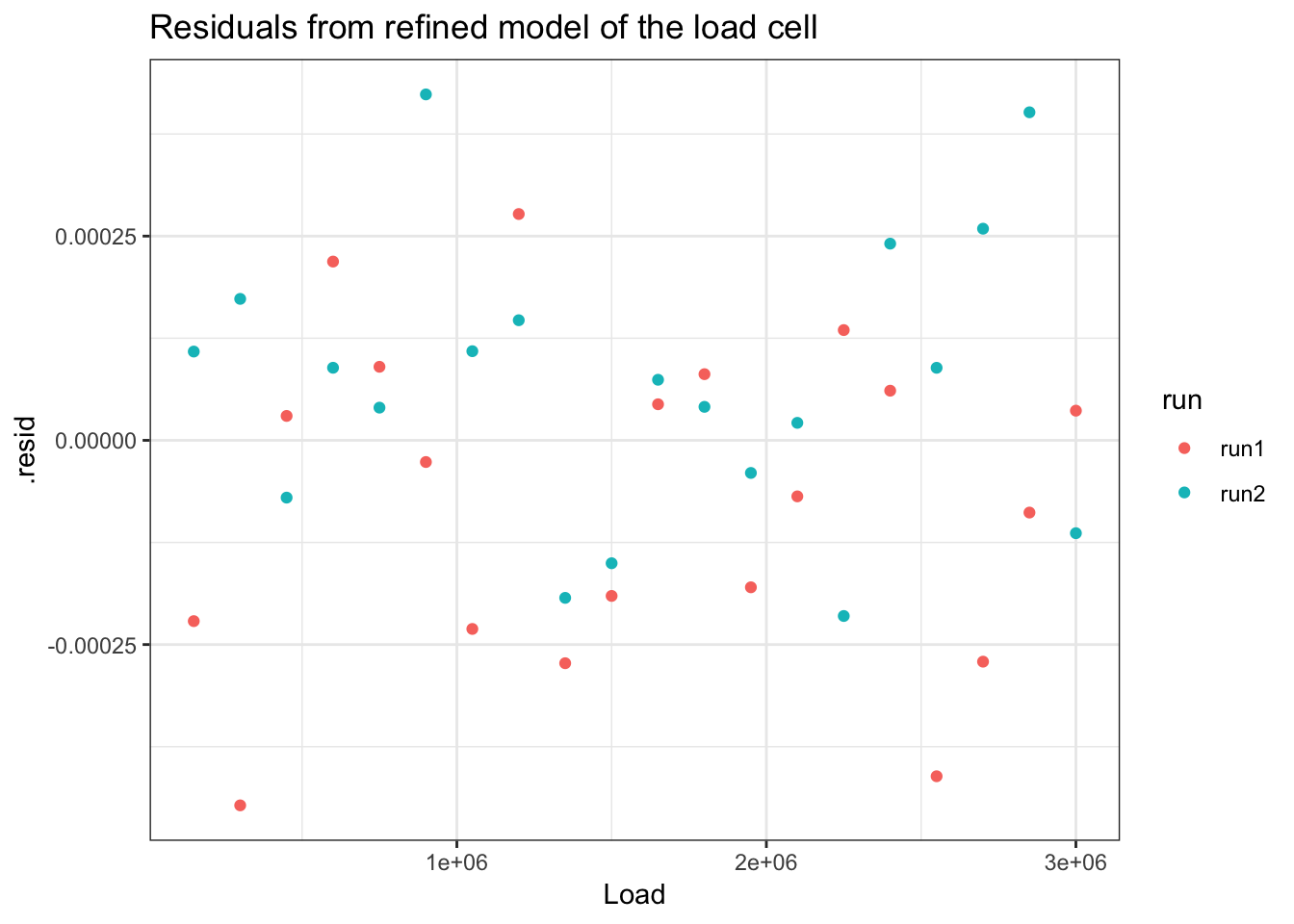
4.4 Applying models to multiple datasets
4.4.1 Revisting the Ascombe dataset
x_anscombe <- anscombe %>%  # results will be storred into a new object x_anscombe; we start with the original data frame "anscombe"
  dplyr::select(x1, x2, x3, x4) %>%  # select the columns we want to work with
  rename(group1 = x1, group2 = x2, group3 = x3, group4 = x4) %>% # rename the values using a generic header
  gather(key = group, value = x_values, group1, group2, group3, group4) # gather the columns into rows

x_anscombe
## group x_values
## 1 group1 10
## 2 group1 8
## 3 group1 13
## 4 group1 9
## 5 group1 11
## 6 group1 14
## 7 group1 6
## 8 group1 4
## 9 group1 12
## 10 group1 7
## 11 group1 5
## 12 group2 10
## 13 group2 8
## 14 group2 13
## 15 group2 9
## 16 group2 11
## 17 group2 14
## 18 group2 6
## 19 group2 4
## 20 group2 12
## 21 group2 7
## 22 group2 5
## 23 group3 10
## 24 group3 8
## 25 group3 13
## 26 group3 9
## 27 group3 11
## 28 group3 14
## 29 group3 6
## 30 group3 4
## 31 group3 12
## 32 group3 7
## 33 group3 5
## 34 group4 8
## 35 group4 8
## 36 group4 8
## 37 group4 8
## 38 group4 8
## 39 group4 8
## 40 group4 8
## 41 group4 19
## 42 group4 8
## 43 group4 8
## 44 group4 8y_anscombe <- anscombe %>%
dplyr::select(y1, y2, y3, y4) %>%
gather(key = group, value = y_values, y1, y2, y3, y4) %>% # I don't need to rename the columns as I will discard them (I only need one column to indicate the group number)
dplyr::select(y_values)
y_anscombe## y_values
## 1 8.04
## 2 6.95
## 3 7.58
## 4 8.81
## 5 8.33
## 6 9.96
## 7 7.24
## 8 4.26
## 9 10.84
## 10 4.82
## 11 5.68
## 12 9.14
## 13 8.14
## 14 8.74
## 15 8.77
## 16 9.26
## 17 8.10
## 18 6.13
## 19 3.10
## 20 9.13
## 21 7.26
## 22 4.74
## 23 7.46
## 24 6.77
## 25 12.74
## 26 7.11
## 27 7.81
## 28 8.84
## 29 6.08
## 30 5.39
## 31 8.15
## 32 6.42
## 33 5.73
## 34 6.58
## 35 5.76
## 36 7.71
## 37 8.84
## 38 8.47
## 39 7.04
## 40 5.25
## 41 12.50
## 42 5.56
## 43 7.91
## 44 6.89anscombe_tidy <- bind_cols(x_anscombe, y_anscombe)
anscombe_tidy## group x_values y_values
## 1 group1 10 8.04
## 2 group1 8 6.95
## 3 group1 13 7.58
## 4 group1 9 8.81
## 5 group1 11 8.33
## 6 group1 14 9.96
## 7 group1 6 7.24
## 8 group1 4 4.26
## 9 group1 12 10.84
## 10 group1 7 4.82
## 11 group1 5 5.68
## 12 group2 10 9.14
## 13 group2 8 8.14
## 14 group2 13 8.74
## 15 group2 9 8.77
## 16 group2 11 9.26
## 17 group2 14 8.10
## 18 group2 6 6.13
## 19 group2 4 3.10
## 20 group2 12 9.13
## 21 group2 7 7.26
## 22 group2 5 4.74
## 23 group3 10 7.46
## 24 group3 8 6.77
## 25 group3 13 12.74
## 26 group3 9 7.11
## 27 group3 11 7.81
## 28 group3 14 8.84
## 29 group3 6 6.08
## 30 group3 4 5.39
## 31 group3 12 8.15
## 32 group3 7 6.42
## 33 group3 5 5.73
## 34 group4 8 6.58
## 35 group4 8 5.76
## 36 group4 8 7.71
## 37 group4 8 8.84
## 38 group4 8 8.47
## 39 group4 8 7.04
## 40 group4 8 5.25
## 41 group4 19 12.50
## 42 group4 8 5.56
## 43 group4 8 7.91
## 44 group4 8 6.89ggplot(anscombe_tidy, aes(x_values, y_values)) +
geom_line(aes(group = group))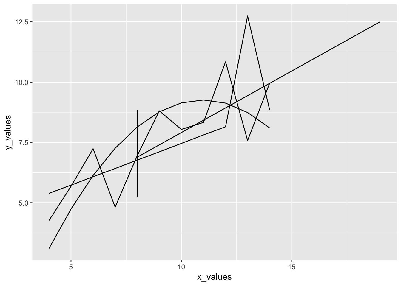
In chapter 1, we constructed models for each group; however, for large datasets, we’d like to be able to streamline this process.
Following the example from chapter 11 of Hadley Wickham:
anscombe_models <- anscombe_tidy %>%
  group_by(group) %>%
  do(mod = lm(y_values ~ x_values, data = ., na.action = na.exclude
     )) %>%
  ungroup()

anscombe_models
## # A tibble: 4 x 2
## group mod
## * <chr> <list>
## 1 group1 <S3: lm>
## 2 group2 <S3: lm>
## 3 group3 <S3: lm>
## 4 group4 <S3: lm>4.4.2 Model-level summaries
model_summary <- anscombe_models %>%
  rowwise() %>%
  glance(mod)

model_summary
## # A tibble: 4 x 12
## # Groups: group [4]
## group r.squared adj.r.squared sigma statistic p.value df logLik AIC
## <chr> <dbl> <dbl> <dbl> <dbl> <dbl> <int> <dbl> <dbl>
## 1 grou… 0.667 0.629 1.24 18.0 0.00217 2 -16.8 39.7
## 2 grou… 0.666 0.629 1.24 18.0 0.00218 2 -16.8 39.7
## 3 grou… 0.666 0.629 1.24 18.0 0.00218 2 -16.8 39.7
## 4 grou… 0.667 0.630 1.24 18.0 0.00216 2 -16.8 39.7
## # … with 3 more variables: BIC <dbl>, deviance <dbl>, df.residual <int>4.4.3 Coefficient-level summaries
coefficient_summary <- anscombe_models %>%
  rowwise() %>%
  tidy(mod)

coefficient_summary
## # A tibble: 8 x 6
## # Groups: group [4]
## group term estimate std.error statistic p.value
## <chr> <chr> <dbl> <dbl> <dbl> <dbl>
## 1 group1 (Intercept) 3.00 1.12 2.67 0.0257
## 2 group1 x_values 0.500 0.118 4.24 0.00217
## 3 group2 (Intercept) 3.00 1.13 2.67 0.0258
## 4 group2 x_values 0.5 0.118 4.24 0.00218
## 5 group3 (Intercept) 3.00 1.12 2.67 0.0256
## 6 group3 x_values 0.500 0.118 4.24 0.00218
## 7 group4 (Intercept) 3.00 1.12 2.67 0.0256
## 8 group4 x_values 0.500 0.118 4.24 0.002164.4.4 Observation Data
observation_summary <- anscombe_models %>%
  rowwise() %>%
  augment(mod)

observation_summary
## # A tibble: 44 x 10
## # Groups: group [4]
## group y_values x_values .fitted .se.fit .resid .hat .sigma .cooksd
## <chr> <dbl> <dbl> <dbl> <dbl> <dbl> <dbl> <dbl> <dbl>
## 1 grou… 8.04 10 8.00 0.391 0.0390 0.1 1.31 6.14e-5
## 2 grou… 6.95 8 7.00 0.391 -0.0508 0.1 1.31 1.04e-4
## 3 grou… 7.58 13 9.50 0.601 -1.92 0.236 1.06 4.89e-1
## 4 grou… 8.81 9 7.50 0.373 1.31 0.0909 1.22 6.16e-2
## 5 grou… 8.33 11 8.50 0.441 -0.171 0.127 1.31 1.60e-3
## 6 grou… 9.96 14 10.0 0.698 -0.0414 0.318 1.31 3.83e-4
## 7 grou… 7.24 6 6.00 0.514 1.24 0.173 1.22 1.27e-1
## 8 grou… 4.26 4 5.00 0.698 -0.740 0.318 1.27 1.23e-1
## 9 grou… 10.8 12 9.00 0.514 1.84 0.173 1.10 2.79e-1
## 10 grou… 4.82 7 6.50 0.441 -1.68 0.127 1.15 1.54e-1
## # … with 34 more rows, and 1 more variable: .std.resid <dbl>ggplot(observation_summary, aes(.se.fit, fill = group)) +
geom_histogram(bins = 50) +
facet_wrap(~ group)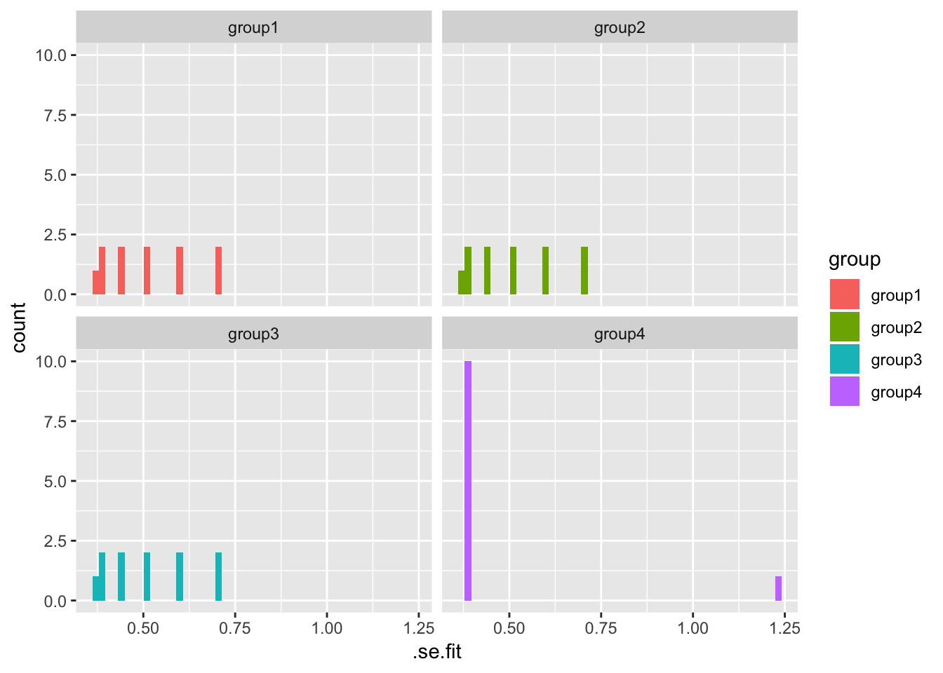
Having model information for each dataset can make the overall analysis much more efficient.