Week 3 Simulations
Can we evaluate and test models without empirical data? Yes, we can generate data given model and experimental design and then observe how a model predicts behavioral patterns. Unlike what we did in week2 (i.e., generate data with rbinom, we will build up our own models (i.e., sequential-sampling models) and see how the choice patterns look like given each model.
In the next few sections, you will build up four sequential-sampling models, which assume a decision is formed through evidence accumulation until accumulated evidence reaches a threshold
(see Figure 3.1). In these four models, we will see how different sets of parameters are used to explain or predict decision-making (i.e., RT).
Here is the overview of four models:
Model1: Sequential-sampling model (without trial-based variability).
Model2: Sequential-sampling model (with trial-based variability).
Model3: Sequential-sampling (Two accumulators)
Model4: Sequential-sampling (One accumulator with Two thresholds)
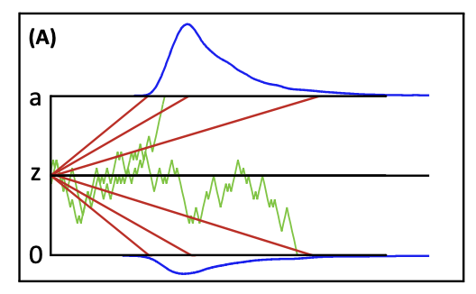
Figure 3.1: Graphical illuscation of simple sequential sampling model. Farrell and Lewandowsky, 2018
A quick note: Set up the environment for your data analysis as usual.
- Change your working directory to Desktop/CMcourse.
- Open a R script and save it as Week3_[First and Last name].R in the current folder.
- Write few comments on the first few rows of your R script. For instance:
# Week 3: Simulation
# First and Last name
# date
- Clean up working environment panel AND plot window before you run the code. This step helps programmers to minimize the chance of using non-interested variables and increase the chance to find out the variables of interest.
# clear working environment panel
rm(list=ls())
From now on, you can copy and paste my code from here to your own R script. Run them (line-by-line using Ctrl+Enter in Windows/Linux or Command+Enter in Mac) and observe changes in the Environment panel (Top-Right) or Files/Plots (Bottom-Right).
Also, if you have time, please replace “values” in the code and see how the results are changed. Ideally, you will see following three statements from the sequential sampling models (Gluth & Laura, in press):
(i) Decisions take time, because sampling happens sequentially.
(ii) The speed of evidence accumulation is influenced by task difficult. More difficult, slower decision.
(iii) Important decision takes time because the desired level of certainty (threshold) is higher.
3.1 Model1: Random-walk model (without trial-based variability)
In the random-walk model, at least two parameters are needed. They are drift rate (v) and threshold (a).
However, knowing the names and meanings of those parameters is not sufficient for R to generate data. You need to tell R (or any other programming software) the value of each parameters and how they should be used.
3.1.1 Simulation: Step-by-step
- Determine parameter values
# 1. Determine parameter values
drift_rate <- 0.05  # 0 = noninformative stimulus; >0 = informative
threshold <- 10  # boundary
2. Determine number of time points (e.g., millisecond)
# 2. Determine number of time points
nsamples <- 1000 #Maximum sampling time point (ms)
3. Pre-allocation. Preallocate the size for output of interest.
Here, we are interested in evidence accumulation at each time point.
There are two benefits of using pre-allocation:
a. to avoid misinterpreting results if code is wrong;
b. having pre-create variable can reduce working load for R (i.e., R doesn’t need to create/extend variable when it is generating data)
#3. Pre-allocate the size for output of interest
evidence <- rep(0, 1, nsamples)- Initialize variable(s) and run the algorithm
 # Initialize variables. Initialization is important to make sure timestep starts from 1.
  timestep <- 1

 # Start sampling until evidence reaches threshold
  while (TRUE){
    evidence[timestep+1] <- evidence[timestep] + drift_rate
    if (evidence[timestep+1] >= threshold) return(timestep) # when the accumulated evidence reaches threshold, return an output: timestep as RT
    timestep <- timestep +1 # timestep increases
  }
    RT<-timestep
    RT
## [1] 200#plot trajectories in stimulus-locked manner
plot(evidence[1:RT],type = 'l',xlim = c(0,nsamples), xlab="RTs (ms)", ylab="Accumulated Evidence (unit)",
main="Sampling path")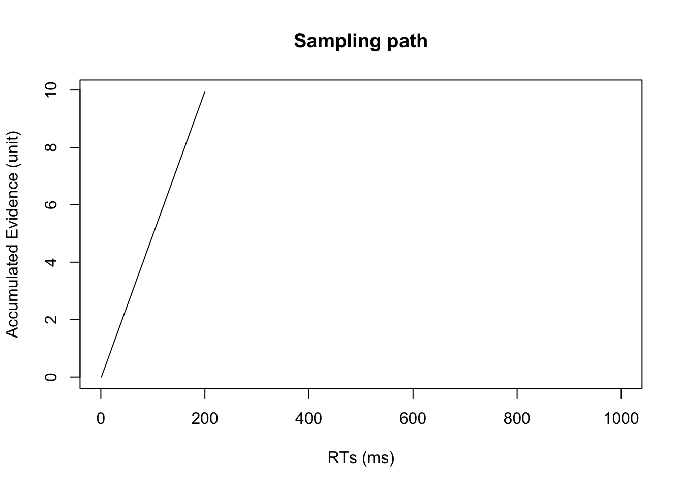
- Create a function that requires drift_rate and threshold as inputs and accumulated evidence as outputs.
# function of model1 (M1)
 model_1 <- function(drift_rate, threshold){
   # Initialize variables. Initialization is important to make sure evidence and timestep start from rationale values.
   # The size of evidence and timestep will not be changed. Instead, these variables will be overwritten over time. Therefore, the size of each variable is not needed to be determined in advance.
   evidence <- 0
   timestep <- 1

   # Start sampling until evidence reaches threshold
   while (TRUE){
     evidence<- evidence + drift_rate
     if (evidence >= threshold) return(timestep) # when the accumulated evidence reaches threshold, return output: timestep as RT
     timestep <- timestep +1
     RT <- timestep
   }
 }
# with the function, we can simulate data for multiple trials (e.g., 1000 trials)
# Determine parameter values
drift_rate <- 0.05
threshold <- 10
# Determine number of trials
n_trial <- 1000
#Pre-allocate the size for output of interest
response_times <- rep(NaN, 1, n_trial)
# run the main script
for (k_trial in 1:n_trial){
response_times[k_trial] <- model_1(drift_rate = drift_rate,
threshold = threshold)
}3.1.2 Visualization
# draw RT distribution as histgram
hist(response_times,xlab="RT (ms)", xlim=c(0, nsamples))
table(response_times)## response_times
## 200
## 10003.2 Model2: Random-walk model (with trial-based variability)
3.2.1 Overview of model2
# main parameters
drift_rate <- 0.05
threshold <- 10
variance <- 0.5

# Initialize variable
timestep <- 1

# Determine number of time points
nsamples <- 1000 #Maximum sampling time point (ms)

#Pre-allocate the size for output of interest
evidence <- rep(0, 1, nsamples)

# Start sampling until evidence reaches threshold
while (TRUE){
  noise = rnorm (mean = 0, sd = variance, n = 1)
  evidence[timestep+1] <- evidence[timestep] + drift_rate + noise
  if (evidence[timestep+1] >= threshold) return(timestep) # when the accumulated evidence reaches threshold
  timestep <- timestep +1
  RT <- timestep
}
#plot trajectories in stimulus-locked manner
plot(evidence[1:RT],type = 'l',xlim = c(0,nsamples), xlab="RTs (ms)", ylab="Accumulated Evidence (unit)", main="Sampling path")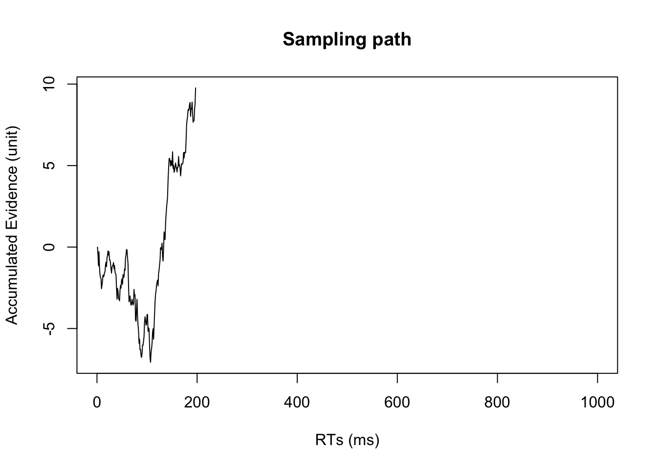
3.2.2 Function
# function of model2 (M2)
model_2 <- function(drift_rate, threshold, variance){
  # Initialize variables. Initialization is important to make sure evidence and timestep start from rationale values.
  evidence <- 0
  timestep <- 1

  # Start sampling until evidence reaches threshold
  while (TRUE){
    noise = rnorm (mean = 0, sd = variance, n = 1)
    evidence <- evidence + drift_rate + noise
    timestep <- timestep +1
    if (evidence >= threshold) return(timestep) # return only one output: timestep
    RT <- timestep
  }
}
3.2.3 Simulation
# with the function, we can simulate data for multiple trials (e.g., 1000 trials)
# determine parameter values
m2.drift_rate <- 0.05
m2.threshold <- 10
m2.variance <-0.5

# Determine number of trials
m2.n_trial <- 1000

#Pre-allocate the size for output of interest
m2.response_times <- rep(NaN, 1, m2.n_trial)

# Start sampling
for (k_trial in 1:m2.n_trial){
  m2.response_times[k_trial] <- model_2(drift_rate = m2.drift_rate,
                                        threshold = m2.threshold,
                                        m2.variance)
}
3.2.4 Visualization
#plot RT distribution
hist(m2.response_times,xlab="RT (ms)", xlim=c(0, nsamples), breaks="FD")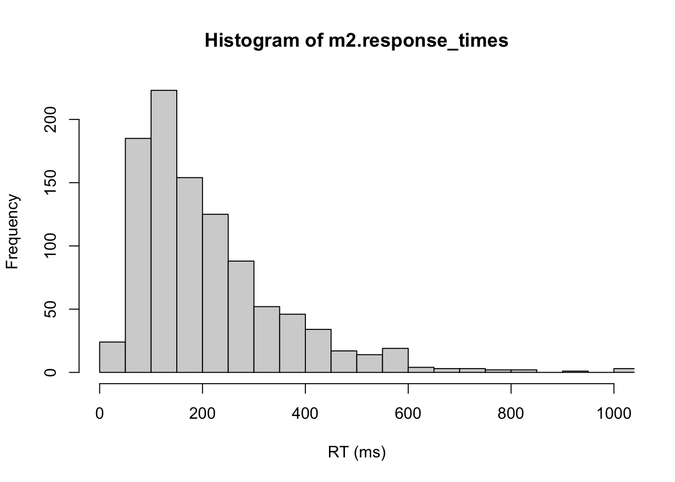
3.3 Model3: Random-walk model (choice between two alternatives)
3.3.1 Function
model_3 <- function(drift_rates, threshold, variance){
   # Initialize variables.
  evidence <- rep(0,length(drift_rates)) # here we have two evidences for two accumulator, separately
  timestep <- 1

   # Start sampling until evidence reaches threshold
  while (TRUE){
    noises <- rnorm (mean = 0, sd = variance, n = length(drift_rates))
    evidence <- evidence + drift_rates + noises
    timestep <- timestep+1
    if (any(evidence >= threshold))
      # Four outputs are returned
      # RT, choice (1 or 2) and accumulated evidence for each option
    return(c(timestep, which(evidence>=threshold & max(evidence)==evidence),evidence))
  }
}
3.3.2 Simulation
# with the function, we can simulate data for multiple trials (e.g., 1000 trials)
# determine parameter values
m3.n_trial <- 10000
m3.drift_rates <- c(0.05,0.025)
m3.threshold <- 10
m3.variance <-0.1

# pre-allocation for the output(s)
m3.response_times <- matrix(,m3.n_trial,4)

# start sampling
for (k_trial in 1:m3.n_trial){
  m3.response_times[k_trial, ] <-model_3(drift_rates = m3.drift_rates,
              threshold = m3.threshold,
              m3.variance)
}
3.3.3 Visualization
We can quickly take a look overall RT distribution
# RTs regardless of choice
hist(m3.response_times[,1],xlab="RT (ms)", xlim=c(0,400), breaks="FD", main="RT distribution of M3")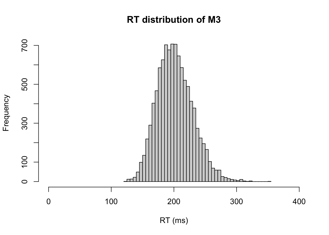
Alternatively, we can separately plot the RT for different actions/choices.
# RTs of Choosing option1
ID.option1 = m3.response_times[,2] == 1
hist(m3.response_times[ID.option1,1],xlab="RT (ms)", xlim=c(0,400), breaks="FD", main="RT distribution of choosing different options", col = c("blue"))

# RTs of Choosing option2
ID.option2 = m3.response_times[,2] == 2
hist(m3.response_times[ID.option2,1],xlab="RT (ms)", col = c("green"), add=T)

# add legend if you plot two data in the same char
legend(1, 400, legend=c("Option1", "Option2"),
       col=c("blue", "green"), fill=c("blue", "green"), cex=0.8)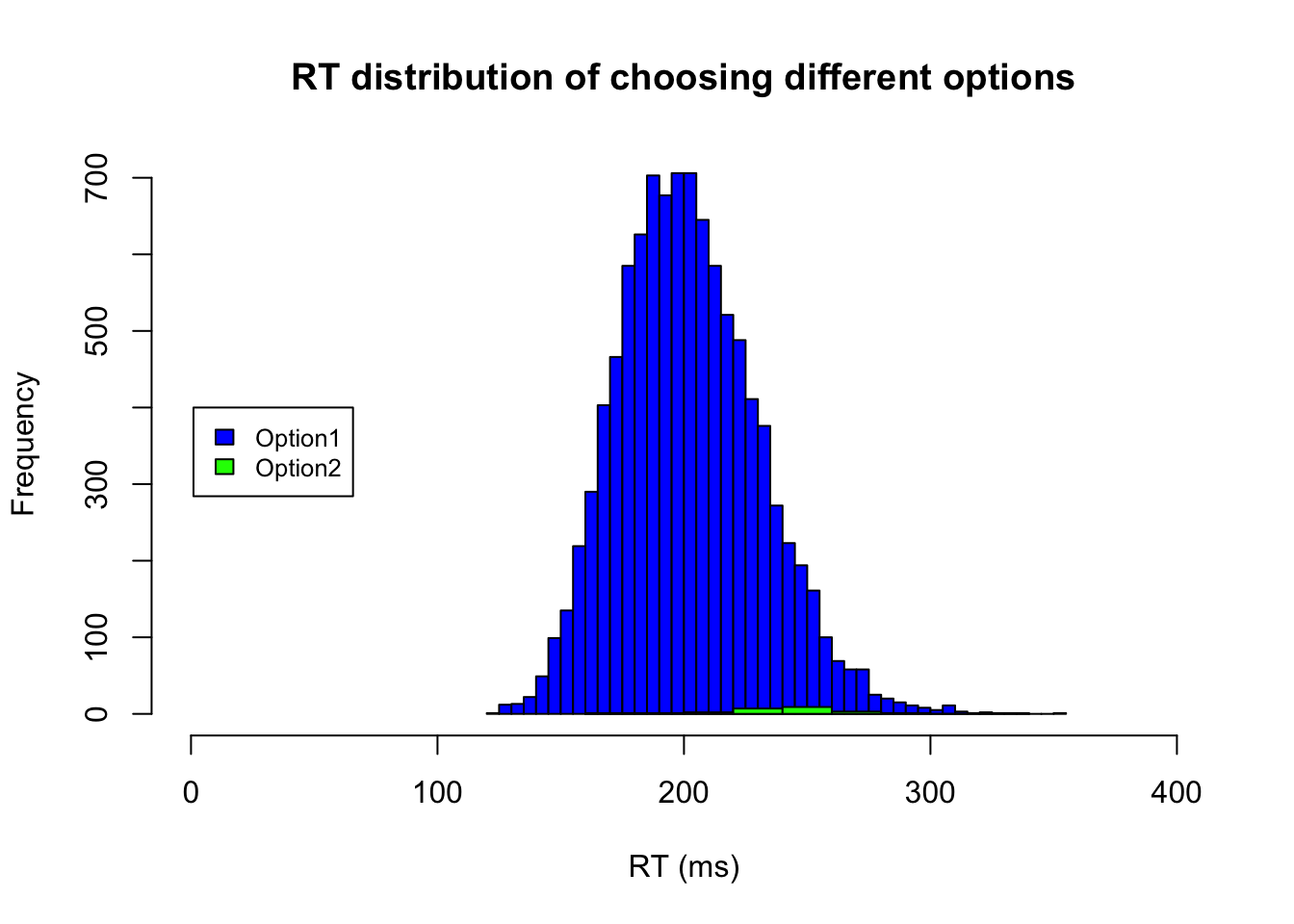
# Zoom in the figure and check RTs of Choosing option2
ID.option2 = m3.response_times[,2] == 2
hist(m3.response_times[ID.option2,1],xlab="RT (ms)", xlim=c(0,400), breaks="FD", main="RT distribution of choosing option2", col = c("green"))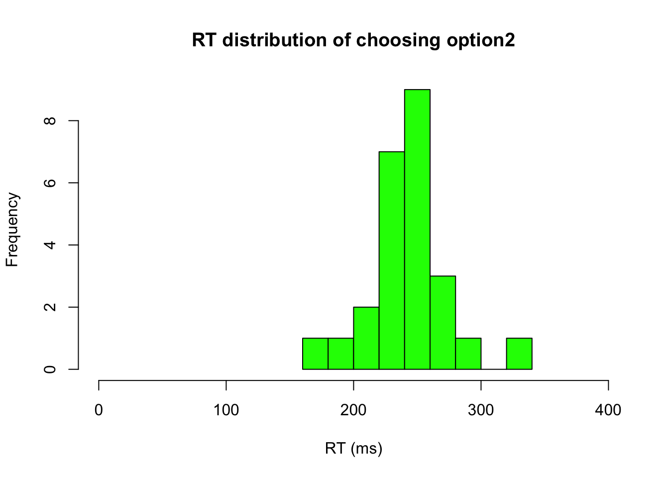
3.4 Model4: Random-walk model (choice between two alternatives and two thresholds)
3.4.1 Function
 model_4 <- function(drift_rate, threshold, variance){
   # Initialize variables.
  evidence <- 0
  timestep <- 1

  # Start sampling until evidence reaches threshold
  while (TRUE){
    noises = rnorm (mean = 0, sd = variance, n = 1)
    evidence <- evidence + drift_rate + noises
    timestep <- timestep +1
    if (abs(evidence) >= threshold)
      return(c(timestep, sign(evidence)))
  }
 }
3.4.2 Simulation
# with the function, we can simulate data for multiple trials (e.g., 1000 trials)
m4.n_trial <- 1000
m4.drift_rate <- 0.05
m4.threshold <- 10
m4.variance <-0.5
m4.response_times <- matrix(0,m4.n_trial,4)
for (k_trial in 1:m4.n_trial){
  m4.response_times[k_trial,] <- model_4(drift_rate = m4.drift_rate,
                                        threshold = m4.threshold,
                                        m4.variance)
}
3.4.3 Visualization
We can quickly take a look overall RT distribution
# RTs distribution
hist(m4.response_times[,1],xlab="RT (ms)", xlim=c(0,800), breaks="FD", main="RT distribution of M4")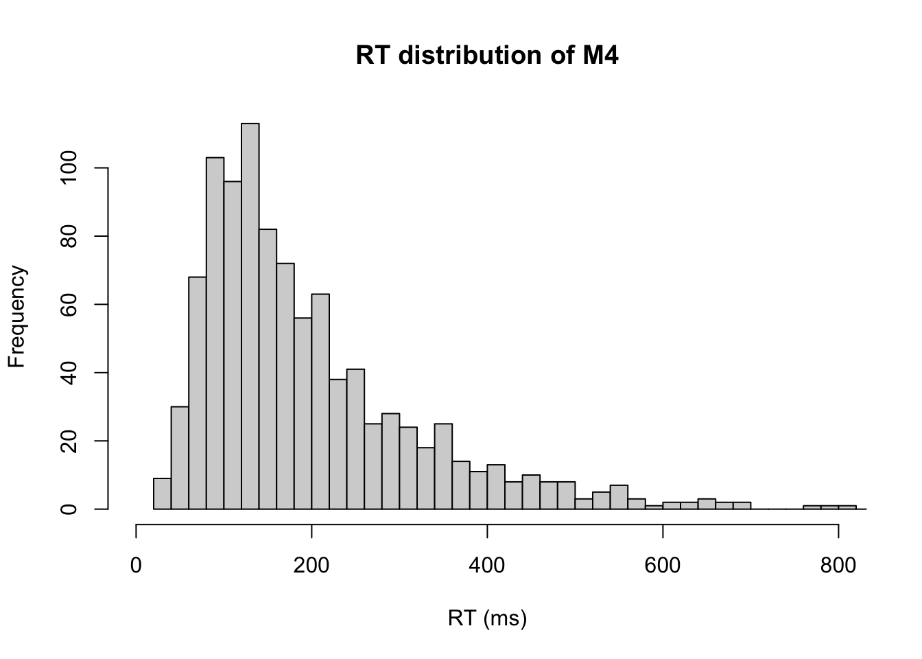 Alternatively, we can separately plot the RT for different actions/choices.
# RTs of Choosing option1
ID.option1 = m4.response_times[,2] == 1
hist(m4.response_times[ID.option1,1],xlab="RT (ms)", xlim=c(0,800), breaks="FD", main="RT distribution of choosing different options", col = c("blue"))

# RTs of Choosing option2
ID.option2 = m4.response_times[,2] == -1
hist(m4.response_times[ID.option2,1],xlab="RT (ms)", col = c("green"), add=T)

# add legend if you plot two data in the same char
legend(600, 150, legend=c("Option1", "Option2"),
       col=c("blue", "green"), fill=c("blue", "green"), cex=0.8)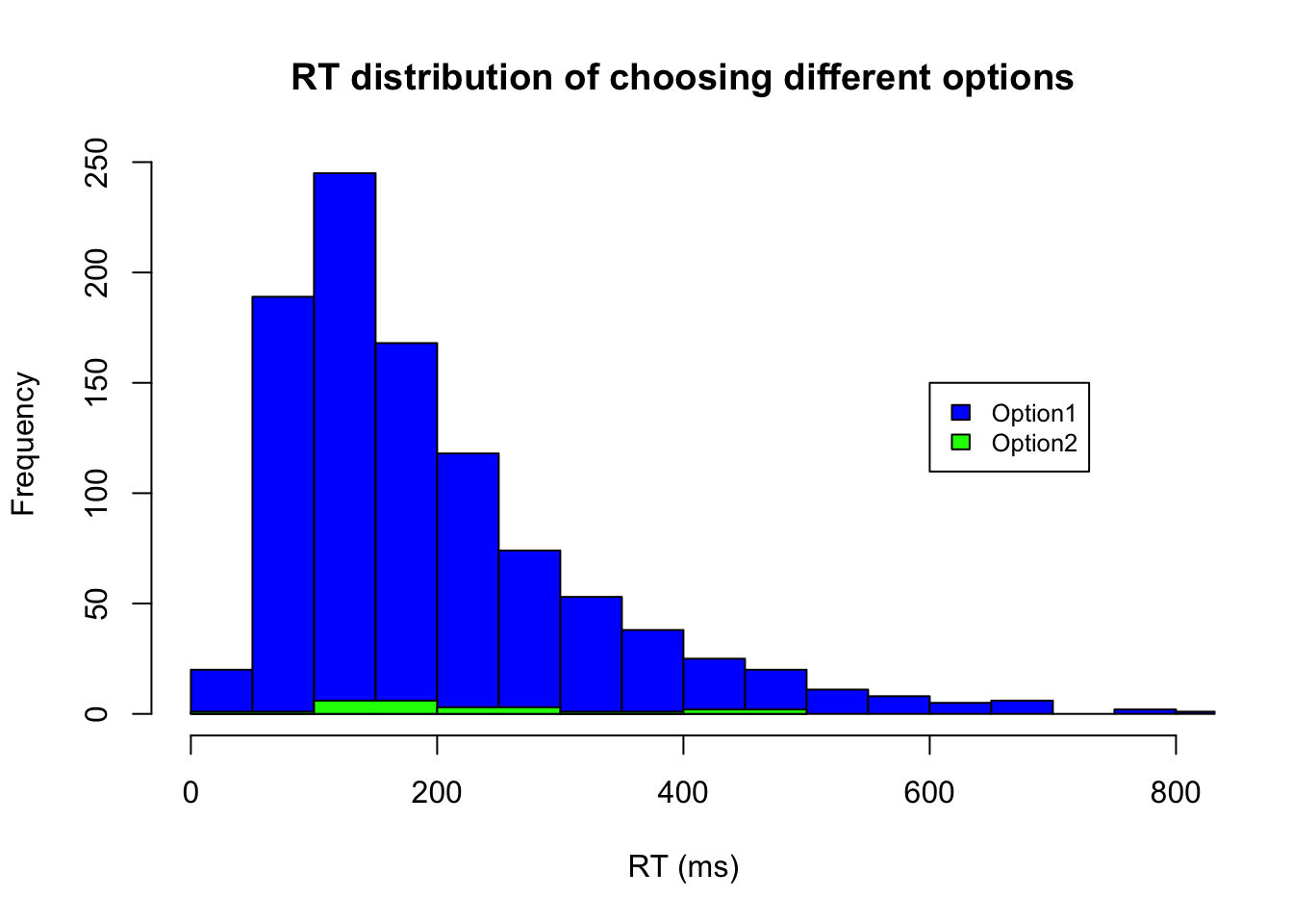
3.5 Exercises
3.5.1 Task A:
Change Variance from 0.5 to 0.1 in the Model2 and summarize the RT and accuracy distribution. What do you observe when you compare the results to the original model2 with Variance of 1? Compute the mean of RT and averaged accuracy rate for both Model2(Variance =0.5) and Model2(Variance =0.1).
3.5.2 Task B:
Increase Threshold from 10 to 5 in the Model4 and summarize the RT and accuracy distribution. What do you observe when you compare the results to the original model4 with threshold of 10? Compute the mean of RT and averaged accuracy rate for both Model4(threshold =10) and Model4(threshold =5). The answers can be found in slides (page title: Simple decision takes time)
3.5.3 Task C: Degub and Add comment to the code
# Example adapted from the textbook (Farrell & Lewandowsky, 2018)
# threshold is 3 and drift rate is 0.03
# Hint1: Four missing lines
# Hint2: try nreps <- 1 to see what happens
nreps <- 1000
nsamples <- 2000

sdrw <- 0.3
t2tsd  <- c(0.0,0.025)

evidence <- matrix(0, nreps, nsamples+1)
for (i in c(1:nreps)) {
  sp <- rnorm(1,0,t2tsd[1])
  dr <- rnorm(1,drift,t2tsd[2])
  evidence[i,] <- cumsum(c(sp,rnorm(nsamples,dr,sdrw)))
  p <-  which(abs(evidence[i,])>criterion)[1]
  responses[i] <- sign(evidence[i,p])
  latencies[i]  <- p
}
hist(latencies)
3.5.4 Task D:
Suppose value difference between two alternatives also contribute to the accumulated evidence.
If there are two conditions: low value difference (|difference| <0.03) and high value difference (0.07>|difference|>0.04) conditions, please create your model5 based on model4 and simulate data for each condition (i.e., 1000 trials and v= 0.5, s= 0.5, a= 10) accordingly. Compute the mean of RT and averaged accuracy rate for each condition.
Hint1: E(t+1) = E(t) + v *(difference) + ε, if |E(t+1)|<a
Hint2: You need to create a list of value differences with, for example, runif.
Hint3: run the model with different condition separately