Exercise 5-1
library(gcookbook)
library(tidyverse)
library(dplyr)
library(ggplot2)
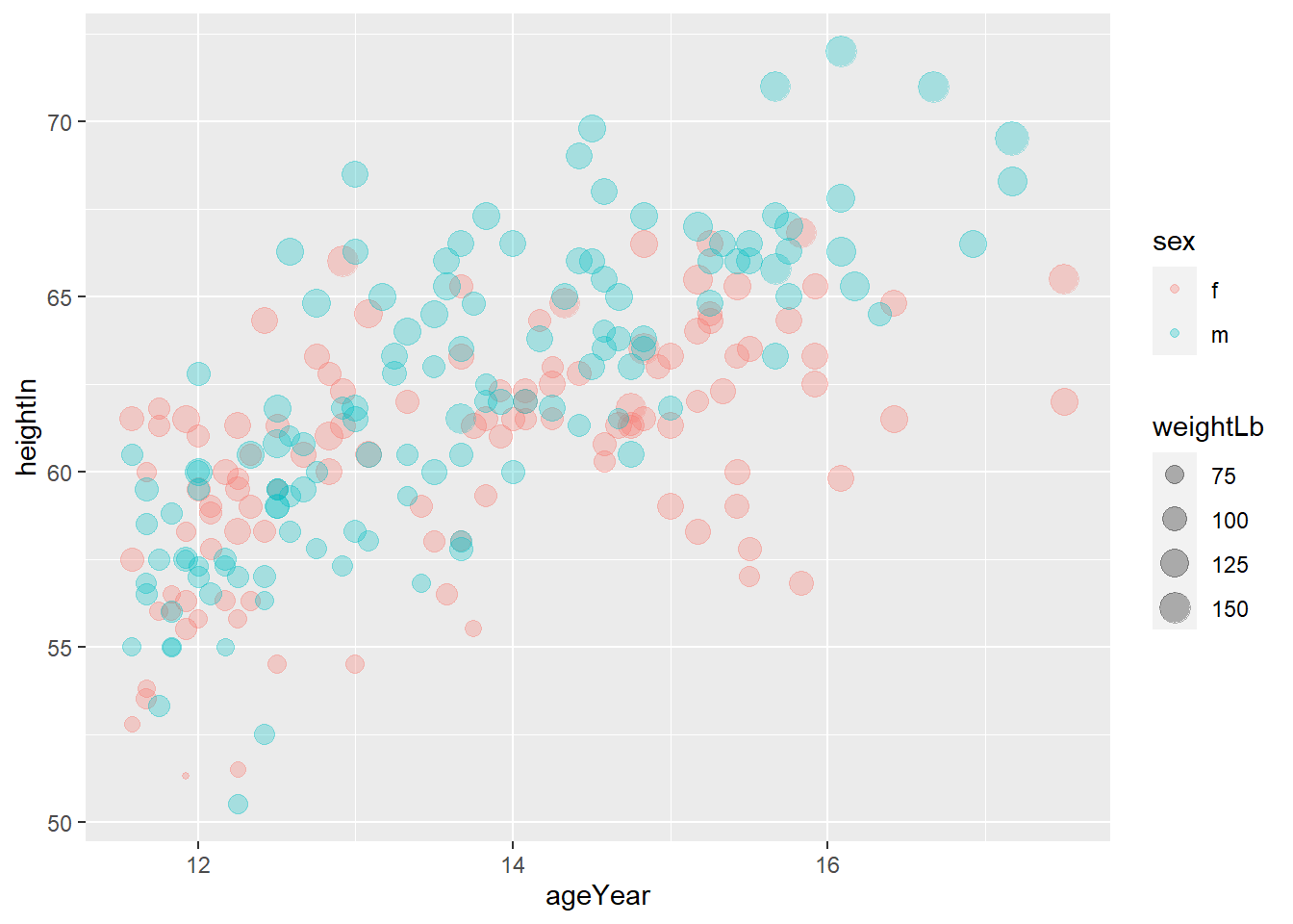
ggplot(heightweight, aes(x=ageYear, y=heightIn, size=weightLb, color=sex))+geom_point()
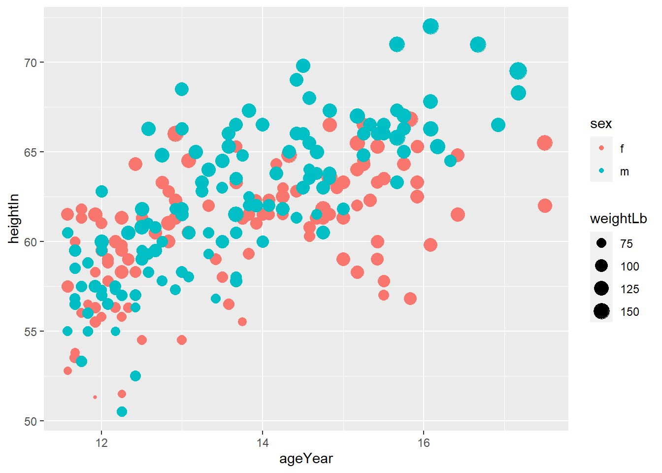
ggplot(heightweight, aes(x=ageYear, y=heightIn, size=weightLb, color=sex))+geom_point(alpha=0.3)
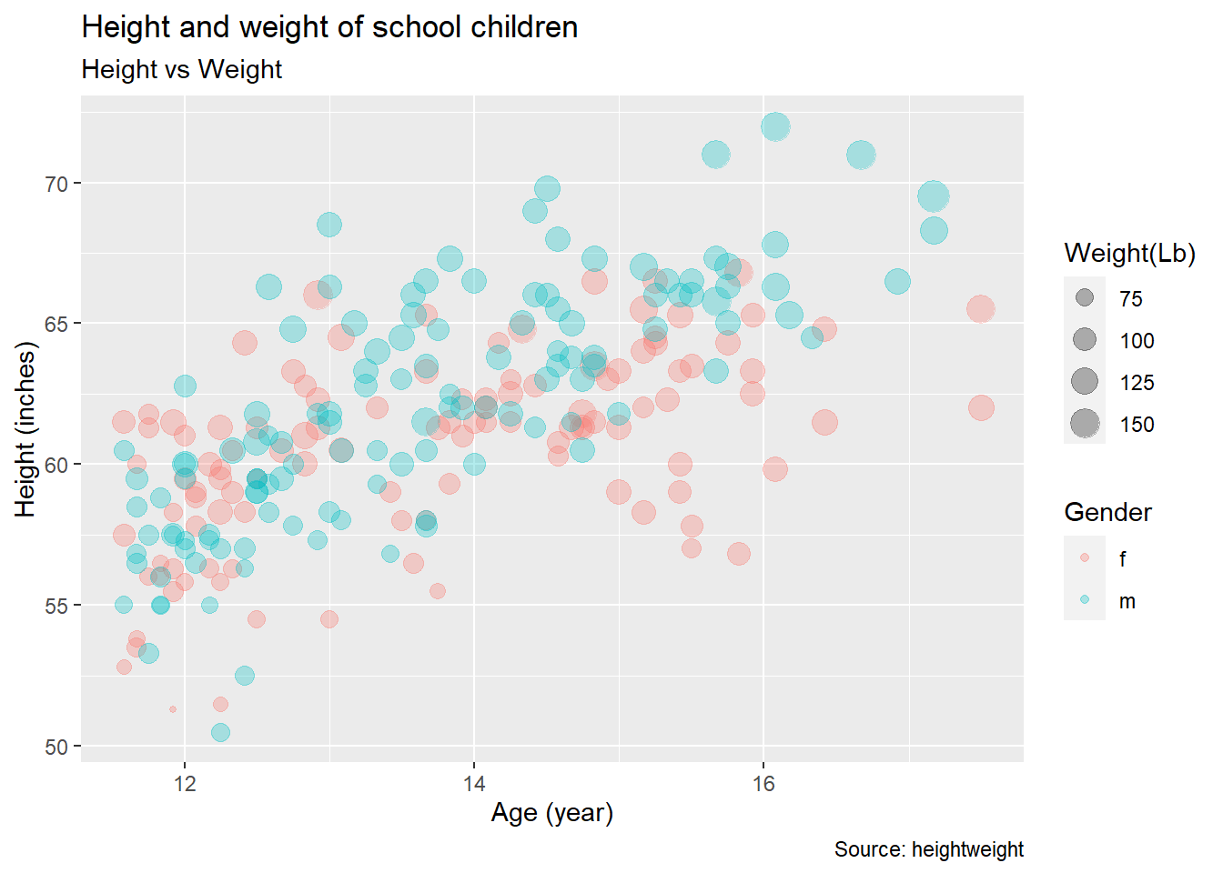
ggplot(heightweight, aes(x=ageYear, y=heightIn, size=weightLb, color=sex))+geom_point(alpha=0.3) +
  labs(title="Height and weight of school children",
       subtitle="Height vs Weight",
       caption="Source: heightweight",
       x="Age (year)",
       y="Height (inches)",
       size="Weight(Lb)",
       color="Gender")
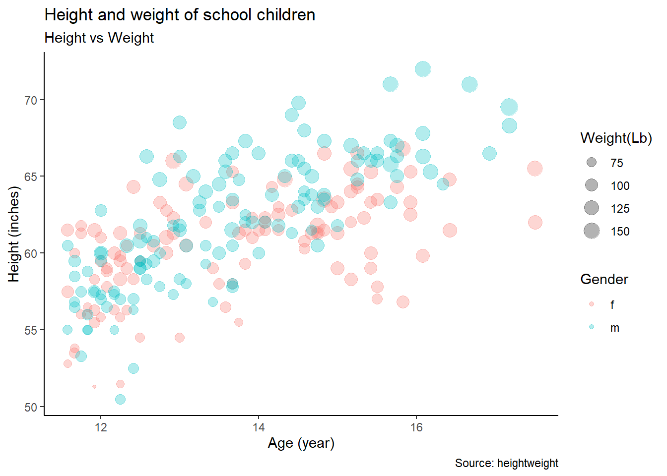
ggplot(heightweight, aes(x=ageYear, y=heightIn, size=weightLb, color=sex))+geom_point(alpha=0.3) +
  labs(title="Height and weight of school children",
       subtitle="Height vs Weight",
       caption="Source: heightweight",
       x="Age (year)",
       y="Height (inches)",
       size="Weight(Lb)",
       color="Gender") + theme_classic()
Exercise 5-2
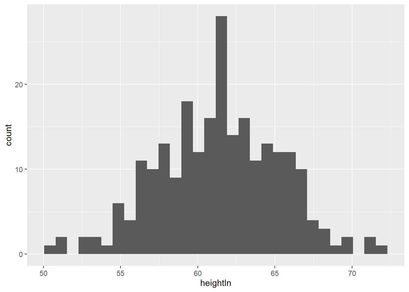
ggplot(heightweight, aes(x=heightIn)) + geom_histogram()
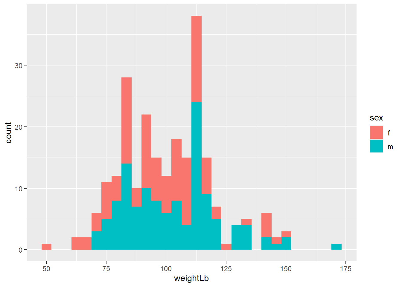
ggplot(heightweight, aes(x=weightLb, fill=sex)) + geom_histogram()
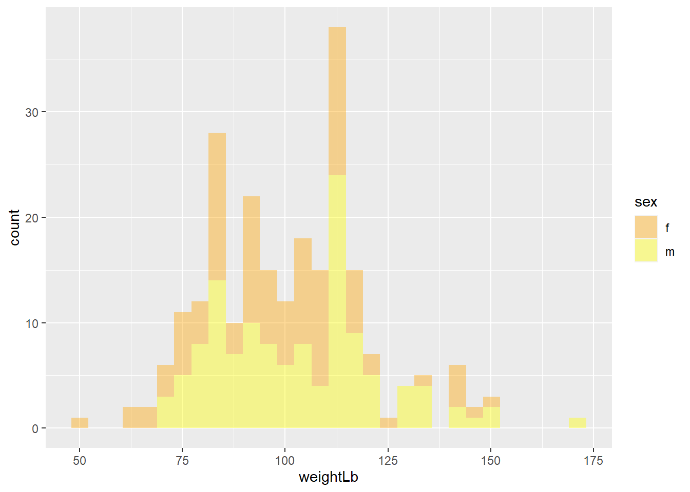
ggplot(heightweight, aes(x=weightLb, fill=sex)) +
  geom_histogram(alpha=0.4) +
  scale_fill_manual(values=c("orange", "yellow"))
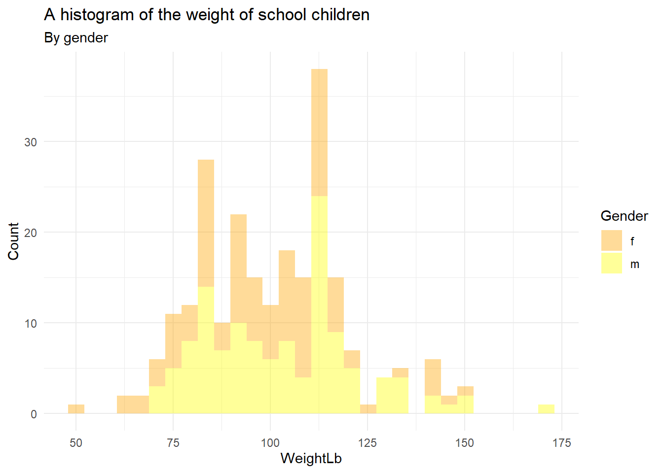
ggplot(heightweight, aes(x=weightLb, fill=sex)) +
  geom_histogram(alpha=0.4) +
  scale_fill_manual(values=c("orange", "yellow")) +
  labs(title = "A histogram of the weight of school children",
       subtitle = "By gender",
       x="WeightLb",
       y="Count",
       fill="Gender") + theme_minimal()
Exercise 5-4
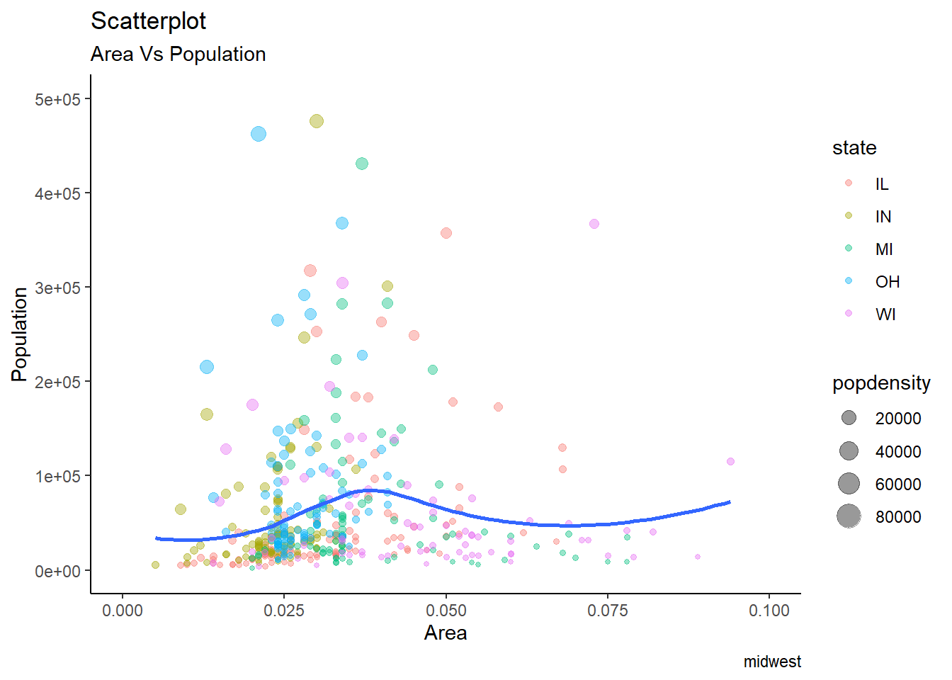
ggplot(midwest, aes(x = area, y = poptotal)) +
  geom_point(alpha=0.4, aes(size = popdensity, color = state)) +
  geom_smooth(se=FALSE) +
  xlim(c(0, 0.1)) +
  ylim(c(0, 500000)) +
  labs(title = "Scatterplot",
       subtitle = "Area Vs Population",
       x = "Area",
       y = "Population",
       caption = "midwest") +
  theme_classic()
## Warning: Removed 15 rows containing non-finite values (stat_smooth).
## Warning: Removed 15 rows containing missing values (geom_point).
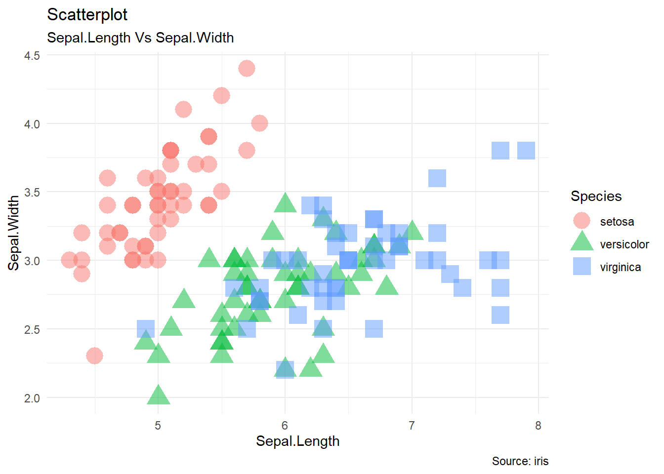
Exercise 5-5
ggplot(iris, aes(x=Sepal.Length, y=Sepal.Width, shape=Species, color=Species)) +
  geom_point(alpha=0.5, size=6) +
  theme_minimal() +
  labs(title = "Scatterplot",
       subtitle = "Sepal.Length Vs Sepal.Width",
       caption = "Source: iris")
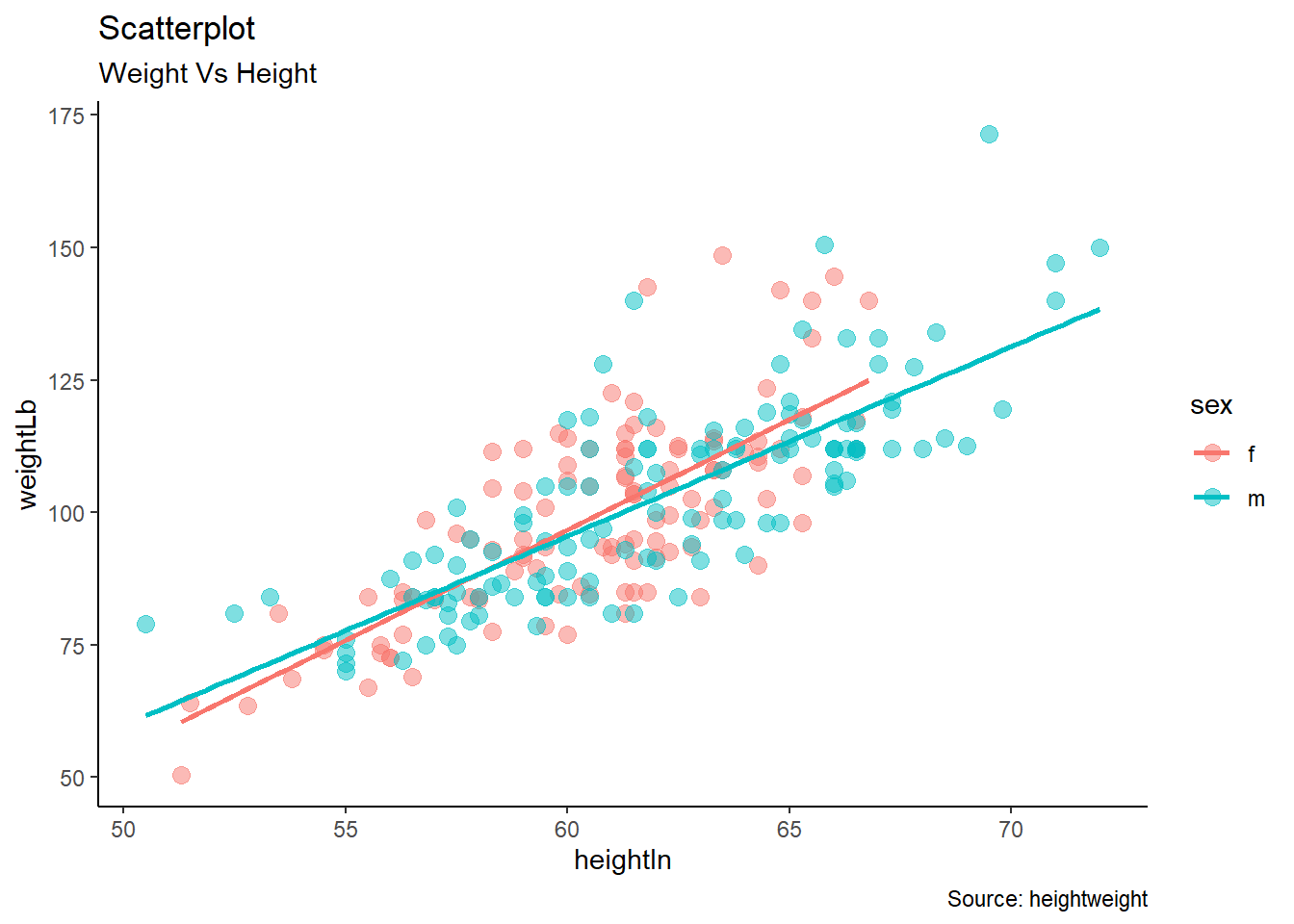
Exercise 5-6
ggplot(heightweight, aes(x=heightIn, y=weightLb, color=sex)) +
  geom_point(alpha=0.5, size=3) +
  geom_smooth(se=FALSE, method="lm") +
  theme_classic() +
  labs(title = "Scatterplot",
       subtitle = "Weight Vs Height",
       caption = "Source: heightweight")
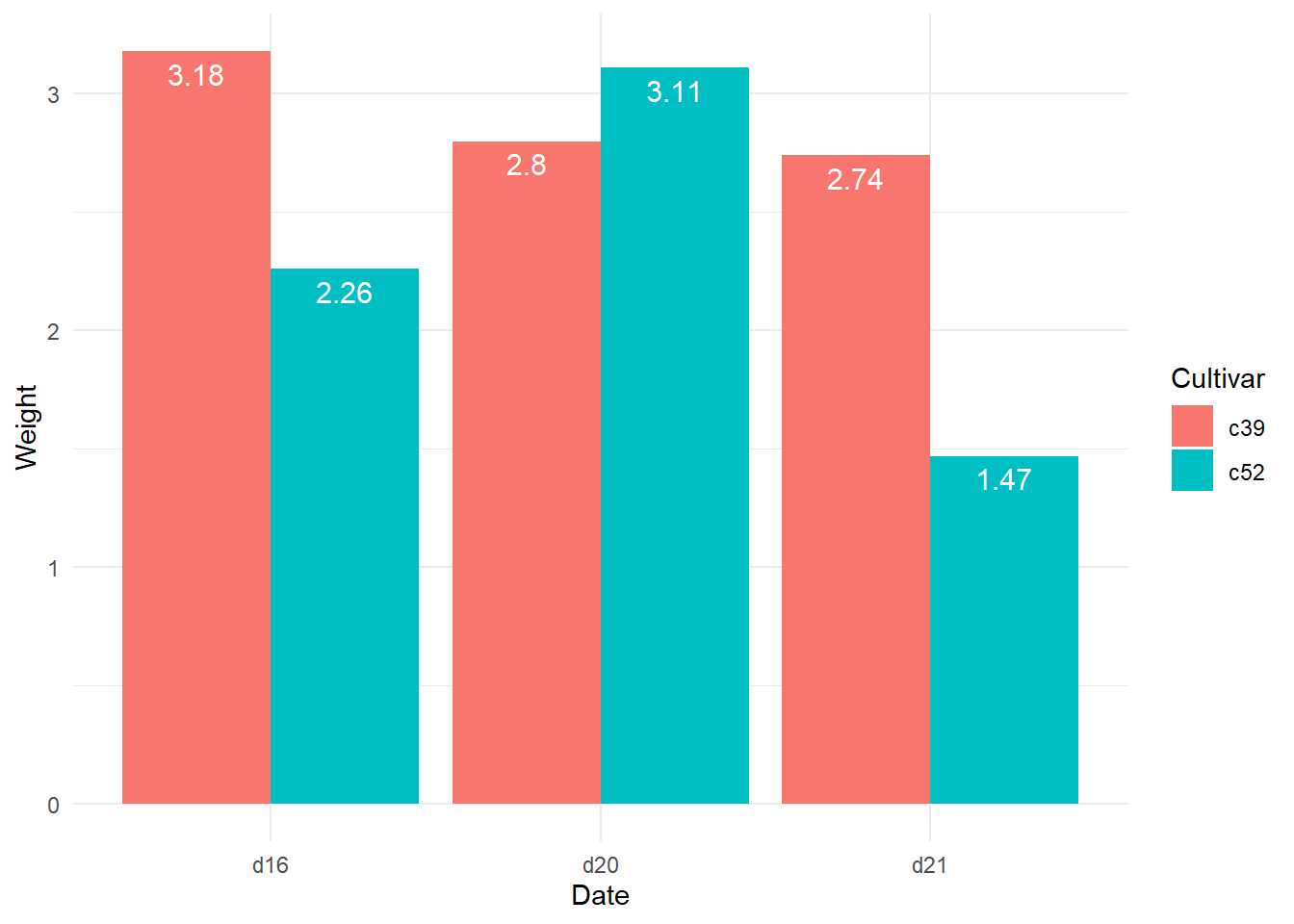
Exercise 5-8
ggplot(cabbage_exp, aes(x=Date, y=Weight, fill=Cultivar)) +
  geom_bar(stat='identity', position="dodge") +
  geom_text(aes(label = Weight), colour = "white", size = 4, vjust = 1.5, position = position_dodge(.9)) +
  theme_minimal()