Chapter 2 Analyzing Instruction with Code

The technical and analyzing part of the project is accomplished through R. Analytical data sets have been pushed into a GitHub repository.

2.1 Library Packages

library(spatstat)
library(here)
library(sp)
library(rgeos)
library(maptools)
library(GISTools)
library(tmap)
library(sf)
library(geojson)
library(geojsonio)
library(tmaptools)
library(tidyverse)
library(stringr)
library(ggplot2)
library(spdep)

2.2 Data Reading

First, get the London Borough Boundaries

LondonBoroughs <- st_read("https://github.com/LingruFeng/GIS_assessment/blob/main/London_Boroughs.gpkg?raw=true")

## Reading layer `london_boroughs' from data source `https://github.com/LingruFeng/GIS_assessment/blob/main/London_Boroughs.gpkg?raw=true' using driver `GPKG'
## Simple feature collection with 33 features and 7 fields
## geometry type:  POLYGON
## dimension:      XY
## bbox:           xmin: 503568.2 ymin: 155850.8 xmax: 561957.5 ymax: 200933.9
## projected CRS:  OSGB 1936 / British National Grid

LondonBoroughs <- LondonBoroughs %>% st_transform(., 27700)

Now get the location of all rapid charging points in the City

charging_points <- st_read("https://github.com/LingruFeng/GIS_assessment/blob/main/Rapid_charging_points.gpkg?raw=true")

## Reading layer `Rapid_charging_points' from data source `https://github.com/LingruFeng/GIS_assessment/blob/main/Rapid_charging_points.gpkg?raw=true' using driver `GPKG'
## Simple feature collection with 156 features and 12 fields
## geometry type:  POINT
## dimension:      XY
## bbox:           xmin: 505012.1 ymin: 157855.5 xmax: 555472.3 ymax: 199091.7
## projected CRS:  unnamed

charging_points <- charging_points %>% st_set_crs(., 27700) %>% st_transform(.,27700)

Get public use points and taxi charging points

taxi <- charging_points %>% filter(taxipublicuses == 'Taxi')
public <- charging_points %>% filter(taxipublicuses == 'Public use' | taxipublicuses == 'Public Use')

2.3 Data Cleaning

select the points inside London

charging_points <- charging_points[LondonBoroughs,]
taxi <- taxi[LondonBoroughs,]
public <- public[LondonBoroughs,]

Correct the borough name to make different data set match each other

LondonBoroughs[22,2]='Hammersmith & Fulham'
LondonBoroughs[19,2]='Richmond'
names(LondonBoroughs)[names(LondonBoroughs) == 'name'] <- 'borough'
public[77,1]='Hillingdon'
taxi[6,1]='City of London'

2.4 Data Summarizing

Summarize the total number of rapid charging points for public use and taxi in each borough

Count the number of rapid charging points for public use in each borough

public_point <- public %>% 
  sf::st_as_sf() %>%
  st_drop_geometry() %>% 
  full_join(LondonBoroughs, by = "borough") %>% 
  select('borough','numberrcpoints')
public_point[is.na(public_point)] <- 0
public_point$numberrcpoints <- as.numeric(public_point$numberrcpoints)
public_point <- public_point %>% group_by(borough) 
public_point <- summarise(public_point,public_point_number=sum(numberrcpoints))

Count the number of rapid charging points for taxi in each borough

taxi_point <- taxi %>% 
  sf::st_as_sf() %>%
  st_drop_geometry() %>% 
  full_join(LondonBoroughs, by = "borough") %>% 
  select('borough','numberrcpoints')
taxi_point[is.na(taxi_point)] <- 0
taxi_point$numberrcpoints <- as.numeric(taxi_point$numberrcpoints)
taxi_point <- taxi_point %>% group_by(borough) 
taxi_point <- summarise(taxi_point,taxi_point_number=sum(numberrcpoints))

Join the summarized data into LondonBoroughs

LondonBoroughs <- LondonBoroughs %>%
  left_join(.,
            public_point, 
            by = "borough") %>%
  left_join(.,
            taxi_point, 
            by = "borough")

Calculate the density of the charging points in each borough

LondonBoroughs <- LondonBoroughs %>%
  mutate(taxi_density = taxi_point_number/hectares*10000) %>%
  mutate(public_density = public_point_number/hectares*10000)

2.5 Data Mapping

Charging site data mapping

tmap_mode("plot")

## tmap mode set to plotting

tm1 <- tm_shape(LondonBoroughs)+ 
  tm_polygons(col="gray",alpha = 0.2)+
  tm_layout(frame=FALSE)+
  tm_shape(public)+
  tm_symbols(col = "red", scale = .4)+
  tm_credits("(a) Public Use", position=c(0.25,0.8), size=2)
tm2 <- tm_shape(LondonBoroughs)+ 
  tm_polygons(col="gray",alpha = 0.2)+
  tm_layout(frame=FALSE)+
  tm_shape(taxi)+
  tm_symbols(col = "blue", scale = .4)+
  tm_credits("(b) Taxi", position=c(0.35,0.8), size=2)+
  tm_scale_bar(text.size=0.85,position=c(0.57,0.14))+
  tm_compass(north=0,position=c(0.8,0.25),size=3)+
  tm_credits("(c) Greater London Authority",position=c(0.53,0.12),size = 1)
t=tmap_arrange(tm1,tm2)
t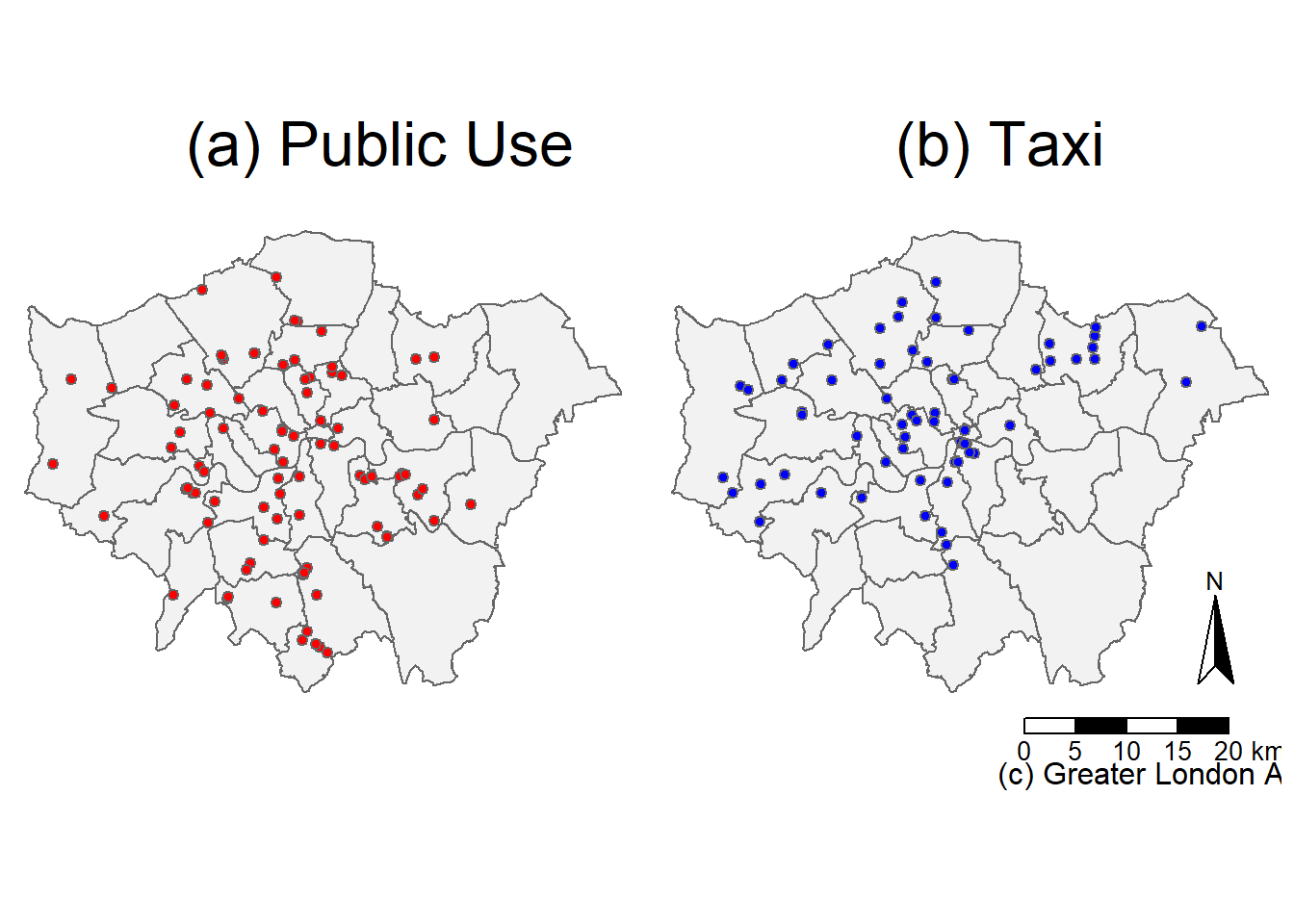

Charging point density mapping

Public use charging point density in boroughs of London

tm3 <- tm_shape(LondonBoroughs) +
  tm_polygons("public_density",
  style="jenks",
  palette=brewer.pal(5, "Reds"),
  midpoint=NA,
  title="Density \n(per 10,000 ha)")+
  tm_layout(frame=FALSE,
            legend.position = c("right","bottom"), 
            legend.text.size=1, 
            legend.title.size = 1.5)+
  tm_scale_bar(text.size=0.85,position=c(0,0.03))+
  tm_compass(north=0,position=c(0.03,0.12),size=3.5,text.size = 1)+
  tm_credits("(c) Greater London Authority",position=c(0,0),size = 1)+
  tm_text("borough", size=1.1,remove.overlap=TRUE,col="black")
tm3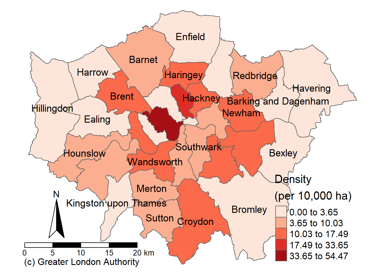

Taxi charging point density in boroughs of London

tm4 <- tm_shape(LondonBoroughs) +
  tm_polygons("taxi_density",
              style="jenks",
              palette=brewer.pal(5, "Blues"),
              midpoint=NA,
              title="Density \n(per 10,000 ha)")+
  tm_layout(frame=FALSE,
            legend.position = c("right","bottom"), 
            legend.text.size=1, 
            legend.title.size = 1.5)+
  tm_scale_bar(text.size=0.85,position=c(0,0.03))+
  tm_compass(north=0,position=c(0.03,0.12),size=3.5,text.size = 1)+
  tm_credits("(c) Greater London Authority",position=c(0,0),size = 1)+
  tm_text("borough", size=1.1,remove.overlap=TRUE,col="black")
tm4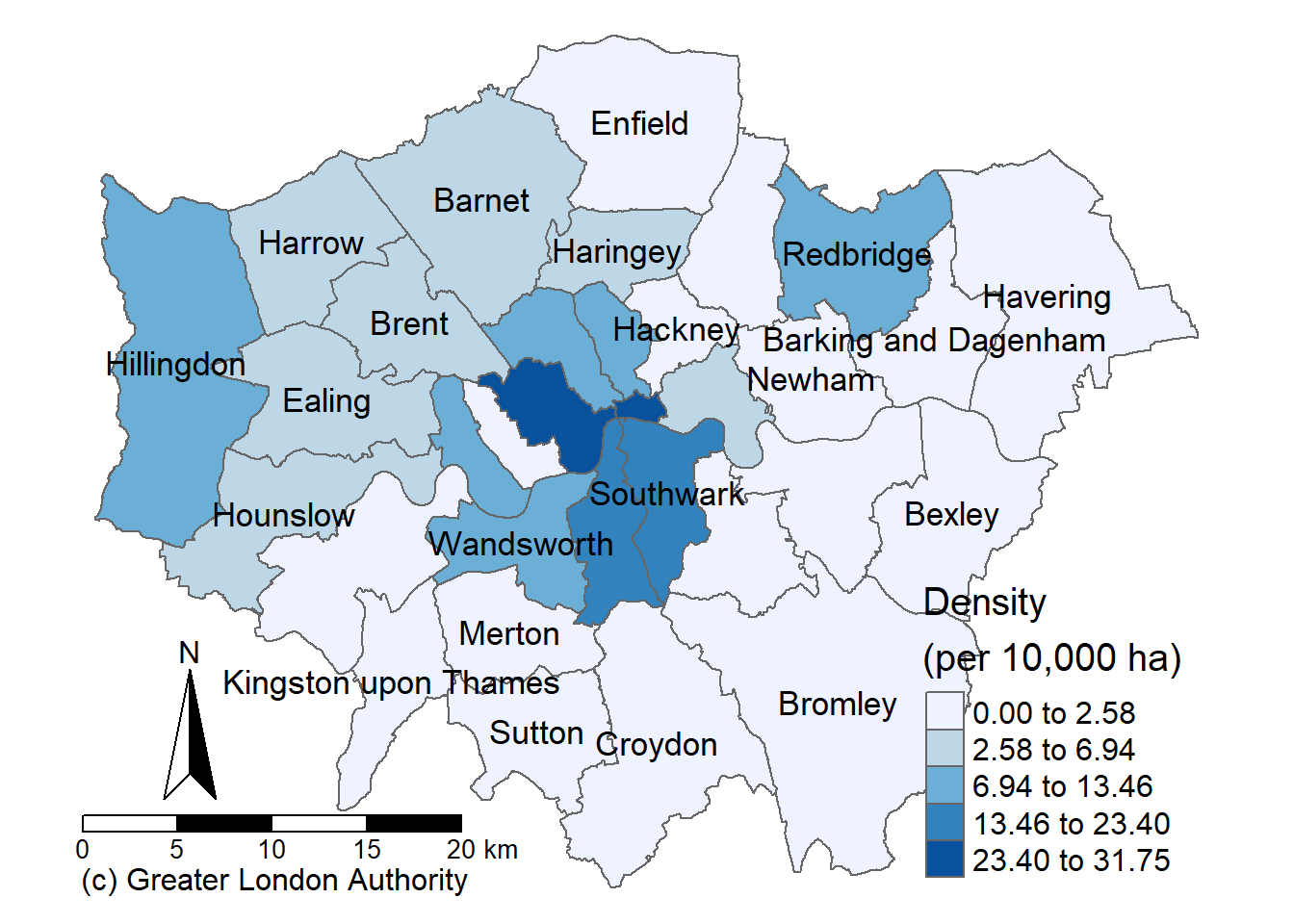

Plot the frequency histogram of Charging point density

taxi_sub <- LondonBoroughs%>%
  st_drop_geometry()%>%
  select(taxi_density) %>%
  mutate(type="taxi")
names(taxi_sub)[names(taxi_sub) == 'taxi_density'] <- 'density'
public_sub <- LondonBoroughs%>%
  st_drop_geometry()%>%
  select(public_density) %>%
  mutate(type="public use")
names(public_sub)[names(public_sub) == 'public_density'] <- 'density'
sub <-rbind(taxi_sub, public_sub)

gghist <- ggplot(sub, aes(x=density, color=type, fill=type)) +
  geom_histogram(position="identity", alpha=0.4,binwidth =4)+
  labs(x="Papid Charging Point Density (per 10,000 ha)",
       y="Frequency")+
  theme_classic()+
  theme(plot.title = element_text(hjust =0.5),
        legend.title = element_text(size =20),
        legend.text = element_text(size = 15),
        axis.title.x =element_text(size=15), 
        axis.title.y=element_text(size=15),)
gghist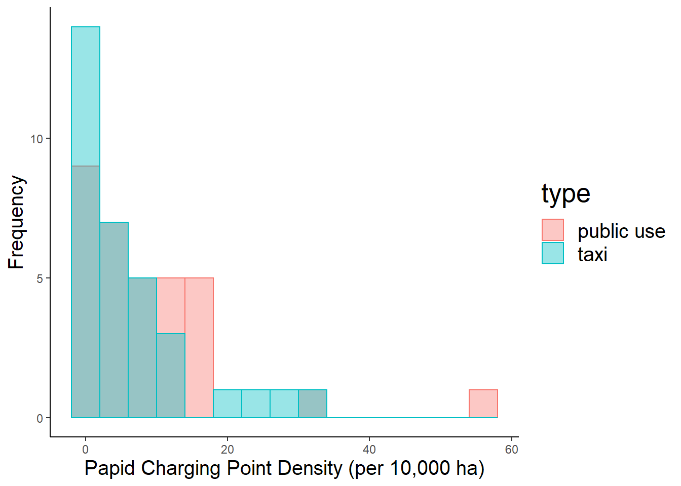

2.6 Charging Site’s Point Pattern Analysis

Do Ripley’s K Tests for both data sets to see if there is any cluster in charging sites

# Set a window as the borough boundary
window <- as.owin(LondonBoroughs)

Ripley’s K Test on Charging Sites for Public Use in London

public<- public %>%
  as(., 'Spatial')

## Warning in showSRID(uprojargs, format = "PROJ", multiline = "NO", prefer_proj
## = prefer_proj): Discarded datum Unknown based on Airy 1830 ellipsoid in CRS
## definition

## Warning in showSRID(SRS_string, format = "PROJ", multiline = "NO", prefer_proj =
## prefer_proj): Discarded datum OSGB 1936 in CRS definition

public.ppp <- ppp(x=public@coords[,1],
                          y=public@coords[,2],
                          window=window)
K <- public.ppp %>%
  Kest(., correction="border") %>%
  plot()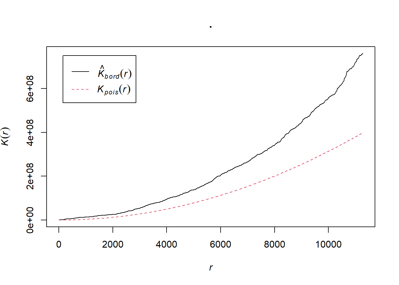

Ripley’s K Test on Charging Sites for Taxi in London

taxi<- taxi %>%
  as(., 'Spatial')

## Warning in showSRID(uprojargs, format = "PROJ", multiline = "NO", prefer_proj
## = prefer_proj): Discarded datum Unknown based on Airy 1830 ellipsoid in CRS
## definition

## Warning in showSRID(SRS_string, format = "PROJ", multiline = "NO", prefer_proj =
## prefer_proj): Discarded datum OSGB 1936 in CRS definition

taxi.ppp <- ppp(x=taxi@coords[,1],
                  y=taxi@coords[,2],
                  window=window)
K <- taxi.ppp %>%
  Kest(., correction="border") %>%
  plot()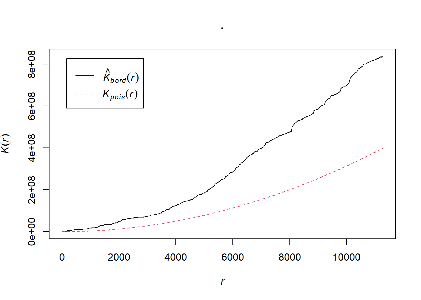

2.7 Global Spatial Autocorrelation Analysis

First calculate the centroids of all Wards in London

coordsW <- LondonBoroughs %>%
  st_centroid()%>%
  st_geometry()

Generate a spatial weights matrix using nearest k-nearest neighbours case

knn_boros <-coordsW %>%
  knearneigh(., k=4) #create a neighbours list of nearest k-nearest neighbours (k=4)
boro_knn <- knn_boros %>%
  knn2nb() %>%
  nb2listw(., style="C")

Analysing Spatial Autocorrelation for both charging point density data set

Moran’s I test (tells us whether we have clustered values (close to 1) or dispersed values (close to -1))

For taxi points’ density

I_global_taxi <- LondonBoroughs %>%
  pull(taxi_density) %>%
  as.vector()%>%
  moran.test(., boro_knn)
I_global_taxi

## 
##  Moran I test under randomisation
## 
## data:  .  
## weights: boro_knn    
## 
## Moran I statistic standard deviate = 3.1165, p-value = 0.0009151
## alternative hypothesis: greater
## sample estimates:
## Moran I statistic       Expectation          Variance 
##        0.28744651       -0.03125000        0.01045746

For public use points’ density

I_global_public <- LondonBoroughs %>%
  pull(public_density) %>%
  as.vector()%>%
  moran.test(., boro_knn)
I_global_public

## 
##  Moran I test under randomisation
## 
## data:  .  
## weights: boro_knn    
## 
## Moran I statistic standard deviate = -0.77738, p-value = 0.7815
## alternative hypothesis: greater
## sample estimates:
## Moran I statistic       Expectation          Variance 
##       -0.10223076       -0.03125000        0.00833709

Geary’s C test (This tells us whether similar values or dissimilar values are cluserting)

For taxi points’ density

C_global_taxi <- 
  LondonBoroughs %>%
  pull(taxi_density) %>%
  as.vector()%>%
  geary.test(., boro_knn)
C_global_taxi

## 
##  Geary C test under randomisation
## 
## data:  . 
## weights: boro_knn 
## 
## Geary C statistic standard deviate = 1.8406, p-value = 0.03284
## alternative hypothesis: Expectation greater than statistic
## sample estimates:
## Geary C statistic       Expectation          Variance 
##        0.77622531        1.00000000        0.01478025

For public use points’ density

C_global_public <- 
  LondonBoroughs %>%
  pull(public_density) %>%
  as.vector()%>%
  geary.test(., boro_knn)
C_global_public

## 
##  Geary C test under randomisation
## 
## data:  . 
## weights: boro_knn 
## 
## Geary C statistic standard deviate = -0.08548, p-value = 0.5341
## alternative hypothesis: Expectation greater than statistic
## sample estimates:
## Geary C statistic       Expectation          Variance 
##        1.01194613        1.00000000        0.01953095

Getis Ord G test(This tells us whether high or low values are clustering.)

For taxi points’ density

G_global_taxi <- 
  LondonBoroughs %>%
  pull(taxi_density) %>%
  as.vector()%>%
  globalG.test(., boro_knn)
G_global_taxi

## 
##  Getis-Ord global G statistic
## 
## data:  . 
## weights: boro_knn 
## 
## standard deviate = 3.6095, p-value = 0.0001534
## alternative hypothesis: greater
## sample estimates:
## Global G statistic        Expectation           Variance 
##       5.339037e-02       3.125000e-02       3.762439e-05

For public use points’ density

G_global_public <- 
  LondonBoroughs %>%
  pull(public_density) %>%
  as.vector()%>%
  globalG.test(., boro_knn)
G_global_public

## 
##  Getis-Ord global G statistic
## 
## data:  . 
## weights: boro_knn 
## 
## standard deviate = -0.37697, p-value = 0.6469
## alternative hypothesis: greater
## sample estimates:
## Global G statistic        Expectation           Variance 
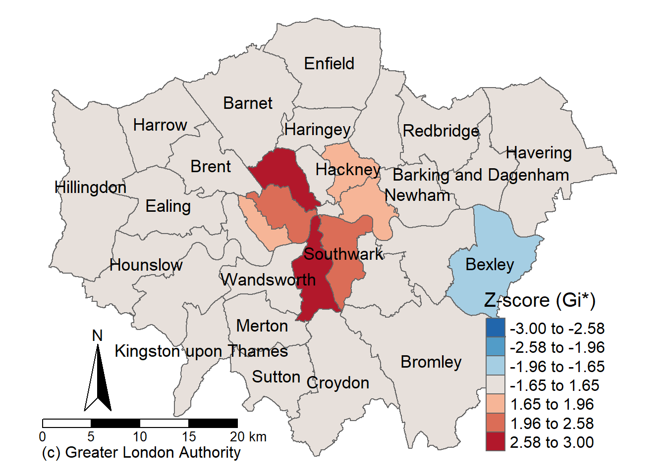
##       2.934219e-02       3.125000e-02       2.561304e-05

2.8 Local Getis-Ord’s G Test

Calculate the Local Getis-Ord’s G z-score for taxi charging point density data

G_local_taxi <- LondonBoroughs %>%
  pull(taxi_density) %>%
  as.vector()%>%
  localG(., boro_knn)

Covert into a dataframe and append into borough data frame

G_local_taxi_df <- data.frame(matrix(unlist(G_local_taxi), nrow=33, byrow=T))
LondonBoroughs_test <- LondonBoroughs %>%
  mutate(z_score = as.numeric(G_local_taxi_df$matrix.unlist.G_local_taxi...nrow...33..byrow...T.))

Plot a map of the local Getis-Ord’s G z-score

# Set the breaks and color bar manually
breaks1<-c(-3.00,-2.58,-1.96,-1.65,1.65,1.96,2.58,3.00)
MoranColours<- rev(brewer.pal(8, "RdBu"))
# Plot the local Getis-Ord’s G test z-score map
tmap_mode("plot")

## tmap mode set to plotting

zscore_taxi <- tm_shape(LondonBoroughs_test) +
  tm_polygons("z_score",
              style="fixed",
              breaks=breaks1,
              palette=MoranColours,
              midpoint=NA,
              title="Z-score (Gi*)")+
  tm_layout(frame=FALSE,
            legend.position = c("right","bottom"), 
            legend.text.size=1, 
            legend.title.size = 1.5)+
  tm_scale_bar(text.size=0.85,position=c(0,0.03))+
  tm_compass(north=0,position=c(0.03,0.12),size=3.5,text.size = 1)+
  tm_credits("(c) Greater London Authority",position=c(0,0),size = 1)+
  tm_text("borough", size=1.1,remove.overlap=TRUE,col="black")
zscore_taxi