Chapter 2 Week 4
2.1 epi.2by2
- Summary measures for count data presented in a 2 by 2 table
library(epiR)
epi.2by2(dat,
         method = c("cohort.count", "cohort.time", "case.control", "cross.sectional"),
         conf.level = 0.95,
         units = 100,
outcome = c("as.columns","as.rows"))dat: an object of classtablecontaining the individual cell frequencies.method: a character string indicating the study design on which the tabular data has been based.- Based on the study design specified by the user, appropriate measures of association, measures of effect in the exposed and measures of effect in the population are returned by the function.
| cohort.count | case.control | |
|---|---|---|
| Measures of association | ||
| RR | \(\checkmark\) | |
| OR | \(\checkmark\) | \(\checkmark\) |
| Measures of effect in the exposed | ||
| ARisk | \(\checkmark\) | \(\checkmark\) |
| AFRisk | \(\checkmark\) | AFest |
| Measures of effect in the population | ||
| PARisk | \(\checkmark\) | \(\checkmark\) |
| PAFRisk | \(\checkmark\) | PAFest |
| chi-squared test | ||
| chisq.strata | \(\checkmark\) | \(\checkmark\) |
| chisq.crude | \(\checkmark\) | \(\checkmark\) |
| chisq.mh | \(\checkmark\) | \(\checkmark\) |
| Mantel-Haenszel (Woolf) test of homogeneity | ||
| RR.homog | \(\checkmark\) | |
| OR.homog | \(\checkmark\) | \(\checkmark\) |
conf.level: magnitude of the returned confidence intervals. The default value is 0.95.units: multiplier for prevalence and incidence (risk or rate) estimates. Default value is 100.unit=1Outcomes per population unitunit=100Outcomes per 100 population unitThe multiplier is applied to Attributable risk, Attributable risk in population, etc.
outcome: how the outcome variable is represented in the contingency table.
2.1.1 Example
# Example in A01
birthwt <- data.frame("Low" = c(21054, 27126), "Normal" = c(14442, 3804294), row.names = c("Dead at Year 1", "Alive at Year 1"))
birthwt
## Low Normal
## Dead at Year 1 21054 14442
## Alive at Year 1 27126 3804294epi.2by2(birthwt,
method = "cohort.count",
conf.level = 0.95,
units = 100,
outcome = "as.rows") # the outcome is represented as rows## Exposed + Exposed - Total
## Outcome + 21054 14442 35496
## Outcome - 27126 3804294 3831420
## Total 48180 3818736 3866916
##
## Point estimates and 95% CIs:
## -------------------------------------------------------------------
## Inc risk ratio 115.55 (113.35, 117.78)
## Odds ratio 204.45 (199.54, 209.49)
## Attrib risk * 43.32 (42.88, 43.76)
## Attrib risk in population * 0.54 (0.53, 0.55)
## Attrib fraction in exposed (%) 99.13 (99.12, 99.15)
## Attrib fraction in population (%) 58.80 (58.28, 59.31)
## -------------------------------------------------------------------
## Test that OR = 1: chi2(1) = 981742.864 Pr>chi2 = <0.001
## Wald confidence limits
## CI: confidence interval
## * Outcomes per 100 population units2.2 chisq.test
- performs chi-squared contingency table tests and goodness-of-fit tests.
chisq.test(x, y = NULL, correct = TRUE,
           p = rep(1/length(x), length(x)), rescale.p = FALSE,
           simulate.p.value = FALSE, B = 2000)
x, y = NULL: the input can be two numeric vectors as x and y (can both be factors), or a matrix as x.correct: a logical indicating whether to apply continuity correction.
2.2.1 output components
chi <- chisq.test(birthwt)
chi
##
## Pearson's Chi-squared test with Yates' continuity correction
##
## data: birthwt
## X-squared = 981695, df = 1, p-value < 2.2e-16# use dollar sign($) to specify output
chi$statistic # the value the chi-squared test statistic## X-squared
## 981695.2chi$parameter # the degrees of freedom## df
## 1chi$p.value## [1] 0chi$method## [1] "Pearson's Chi-squared test with Yates' continuity correction"chi$data.name## [1] "birthwt"chi$observed## Low Normal
## Dead at Year 1 21054 14442
## Alive at Year 1 27126 3804294chi$expected # the expected counts under the null hypothesis## Low Normal
## Dead at Year 1 442.2639 35053.74
## Alive at Year 1 47737.7361 3783682.26chi$residuals # the Pearson residuals, (observed - expected) / sqrt(expected).## Low Normal
## Dead at Year 1 980.10778 -110.08988
## Alive at Year 1 -94.33735 10.59637chi$stdres # standardized residuals, (observed - expected) / sqrt(V)## Low Normal
## Dead at Year 1 990.8294 -990.8294
## Alive at Year 1 -990.8294 990.82942.3 pchisq
- Density, distribution function, quantile function and random generation for the chi-squared (\(\chi^2\)) distribution with
dfdegrees of freedom and optional non-centrality parameterncp.
pchisq(q, df, ncp = 0, lower.tail = TRUE, log.p = FALSE)q: (vector of) quantile(s).df: degrees of freedom (non-negative, but can be non-integer).lower.tail: logical; if TRUE (default), probabilities are \(P[X \le x]\), otherwise, \(P[X > x]\).
2.3.1 Example
To find the p-value that corresponds with a \(\chi^2\) test statistic of 7 from a test with one degree of freedom:
pchisq(7, df=1, lower.tail = FALSE)## [1] 0.008150972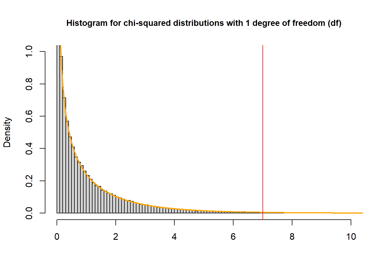
The P-value is the probability of observing a sample statistic as extreme as the test statistic – the area to the left of the red line – “upper” tail
We always set
lower.tail = FALSEwhen calculating P-value of \(\chi^2\) test.Another method to get the p-value
# default: lower.tail = TURE
1 - pchisq(7, df=1)
## [1] 0.008150972