Chapter 1 Some comments on Assignment 7

1.1 Exercise 5.11

Recap:

$$ w_1 = ,w_2 = \ w_1 + w_2 = 1\ E(K_V) = V \ E(K_V) = w_11 + w_22 \ Var(K_V) = ^2_V \ Var(w_1K_1 + w_2K_2) = Var(K_V) = w_1^2Var(K_1)+w2_2Var(K_2)+2w_1w_2Cov(K_1,K_2)\ Var(ax+by) = Var(ax) + Var(by) + 2Cov(ax, by) \ Var(x) = Cov(x,x) \ Var(ax+by) = Var(ax) + Var(by) + 2Cov(ax, by) \ =Cov(ax,ax)+Cov(by,by) + Cov(ax, by) + Cov(by,ax)\ Var({i=1}^n a_ix_i) = Cov({i=1}^na_ix_i, {i=1}^na_ix_i)

Compute the expected return μV and standard deviation $\sigma_V$ of a portfolio consisting of three securities with weights $w_1 = 40\%$, $w_2 = −20\%$, $w_3 = 80\%$, given that the securities have expected returns $\mu_1 = 8\%$, $\mu_2 = 10\%$, $\mu_3 = 6\%$, standard deviations $\sigma_1 = 1.5, \sigma_2 = 0.5, \sigma_3 = 1.2$ and correlations $\rho_{12} = 0.3, \rho_{23} = 0.0, \rho_{31} = −0.2$.

A portfolio constructed from $n$ different securities can be described in terms of their weights:

\[ w_i = \frac{x_iS_i(0)}{V(0)}, \text{for }i = 1,2,\dots,n \]

where $x_i$ is the number of shares of type $i$ in the portfolio, $S_i(0)$ is the initial price of security $i$, and $V(0)$ is the amount initially invested in the portfolio. It will prove convenient to arrange the weights into a one-row matrix

\[ \boldsymbol{w} = [w_1,w_2,\dots,w_n] \]

Linear Algebra:

\[ \boldsymbol{u,v} = \{u_1,u_2,\dots,u_n\} n\times 1 \\ <\boldsymbol{u,v}> = \boldsymbol{u}^T*\boldsymbol{v} = \sum_{i=1}^nu_iv_i\\ (1\times n )* (n\times 1) = 1\times1 = constant\\ [1,3,4]^T*[2,3,4] = 1*2+1*3+1*4+3*2+3*3+3*4+4*2+4*3+4*4 = 72 \]

Just like for two securities, the weights add up to one, which can be written in matrix form as

\[ 1 = \boldsymbol{1}\boldsymbol{w}^T \]

where $\boldsymbol{1}$ is a one-row matrix with all $n$ entries equal to 1, $\boldsymbol{w}^T$ is a one-column matrix, the transpose of $\boldsymbol{w}$, and the usual matrix multiplication rules apply. The attainable set consists of all portfolios with weights $\boldsymbol{w}$ satisfying, called the attainable portfolios.

Suppose that the returns on the securities are $K_1,\dots, K_n.$ The expected returns $\mu_i = E(K_i) \text{ for }i = 1,\dots, n$ will also be arranged into a one-row matrix

\[ m = [\mu_1,\mu_2,\dots,\mu_n] \]

The covariances between returns will be denoted by $c_{ij} = Cov(K_i,K_j)$. They are the entries of the $n\times n$ covariance matrix

\[ \boldsymbol{C}=\begin{bmatrix} c_{11},&c_{12},&\cdots &c_{1n}\\ c_{21},&c_{22},&\cdots &c_{2n}\\ \vdots &\vdots &\ddots &\vdots\\ c_{n1},&c_{n2},&\cdots &c_{nn} \end{bmatrix} \]

Since the covariance matrix is symmetric and positive definite. The diagonal elements are simply the variances of returns, $c_{ii} = Var(K_i)$. In what follows we shall assume, in addition, that $\boldsymbol{C}$ has an inverse $\boldsymbol{C}^{-1}$.

The expected return $\mu_V = E(K_V )$ and variance $\sigma^2_V= Var(K_V )$ of a portfolio with weights $\boldsymbol{w}$ are given by

\[ \begin{aligned} \mu_V &= \boldsymbol{mw}^T \\ \sigma^2_V &= \boldsymbol{wCw}^T \end{aligned} \]

Proof The formula for $\mu_V$ follows by the linearity of expecation:

\[ \mu_V = E(K_V) = E(\sum_{i=1}^nw_iK_i) = \sum_{i=1}^nw_i\sum_{i=1}^nE(K_i) = \sum_{i=1}^nw_i\mu_i = \boldsymbol{mw}^T\\ \sigma^2_V = Var(\sum_{i=1}^nw_iK_i) = Cov(\sum_{i=1}^nw_iK_i, \sum_{j=1}^nw_jK_j) = \sum_{i=1}^n\sum_{j=1}^n w_iw_j c_{ij} = \boldsymbol{wCw}^T \]

For $\sigma^2_V$, we can use the linearity of covariance with respect to each of its arguments:

\[ \begin{aligned} \sigma^2_V &= Var(K_V)\\ &= Var(\sum_{i=1}^nw_iK_i) \end{aligned} \]

\[ Cov(K_1,K_2) = \sigma_1\sigma_2\rho_{12} \]

w = matrix(c(0.4,-0.2,0.8),ncol = 3)
m = matrix(c(0.08,0.1,0.06),ncol = 3)

muV = m%*%t(w)

sigma1 = 1.5
sigma2 = 0.5
sigma3 = 1.2
rho12 = 0.3
rho23 = 0.0
rho31 = -0.2
cov12 = sigma1*sigma2*rho12
cov21 = cov12
cov13 = sigma1*sigma3*rho31
cov31 = cov13
cov23 = sigma2*sigma3*rho23
cov32 = cov23
C = matrix(c(sigma1^2,cov21,cov31,
             cov12,sigma2^2,cov32,
             cov13,cov23,sigma3^2),nrow = 3,ncol = 3)
sigmaV = sqrt(w%*%C%*%t(w))
muV

##      [,1]
## [1,] 0.06

sigmaV

##          [,1]
## [1,] 1.012522

1.2 Exercise 5.17

Suppose that the returns $K_V$ on a given portfolio and $K_M$ on the market portfolio take the following values in different market scenarios:

Scenario	Probability	Return $K_V$	Return $K_M$
$\omega_1$	0.1	−5%	10%
$\omega_2$	0.3	0%	14%
$\omega_3$	0.4	2%	12%
$\omega_4$	0.2	4%	16%

Compute the gradient $\beta_V$ and intercept $\sigma_V$ of the line of best fit.

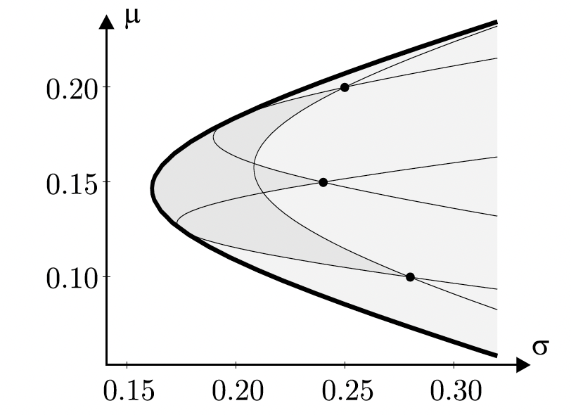
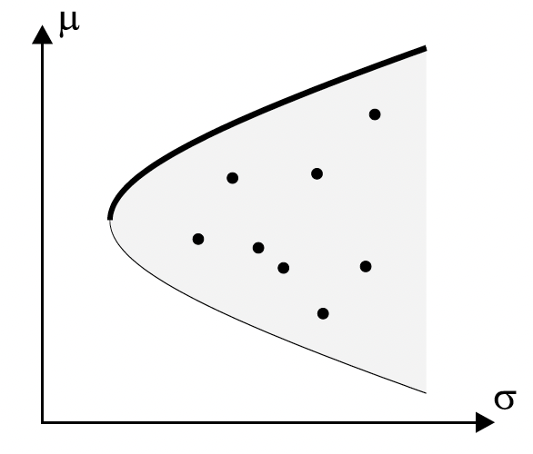
1.2.1 Efficient Frontier

The efficient frontier is the set of optimal portfolios that offer the highest expected return for a defined level of risk or the lowest risk for a given level of expected return. Portfolios that lie below the efficient frontier are sub-optimal because they do not provide enough return for the level of risk. Portfolios that cluster to the right of the efficient frontier are sub-optimal because they have a higher level of risk for the defined rate of return.

The efficient frontier graphically represents portfolios that maximize returns for the risk assumed. Returns are dependent on the investment combinations that make up the portfolio. The standard deviation of a security is synonymous with risk. Ideally, an investor seeks to populate the portfolio with securities offering exceptional returns but whose combined standard deviation is lower than the standard deviations of the individual securities. The less synchronized the securities (lower covariance), the lower the standard deviation. If this mix of optimizing the return versus risk paradigm is successful then that portfolio should line up along the efficient frontier line.

A key finding of the concept was the benefit of diversification resulting from the curvature of the efficient frontier. The curvature is integral in revealing how diversification improves the portfolio’s risk / reward profile. It also reveals that there is a diminishing marginal return to risk. The relationship is not linear. In other words, adding more risk to a portfolio does not gain an equal amount of return. Optimal portfolios that comprise the efficient frontier tend to have a higher degree of diversification than the sub-optimal ones, which are typically less diversified.

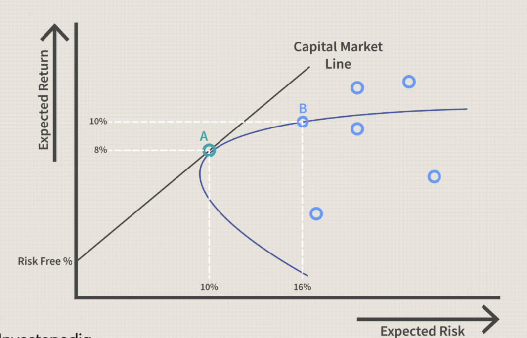
1.2.2 Capital Asset Pricing Model

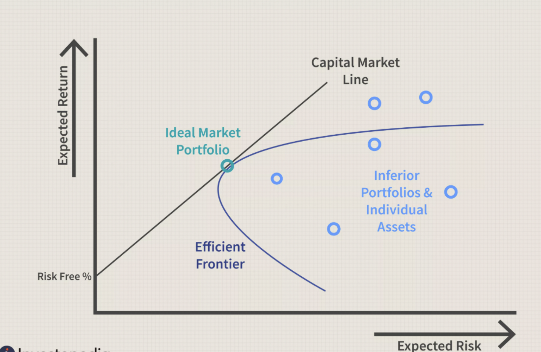
\[ \mu = r_F + \beta*\sigma\\ \beta = (\frac{\mu_M-r_F}{\sigma_M})\\ \mu = r_F + (\frac{\mu_M-r_F}{\sigma_M})\sigma \]

1.2.3 Beta Factor

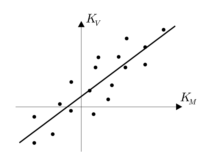
\[ y = \beta_Vx + \alpha_V\\ \text{ordinary least squared (OLS):}\\ min \text{ error} = K_V - y = K_V - (\beta_Vx + \alpha_V) \\ E(error^2) = E(( K_V - (\beta_Vx + \alpha_V))^2) \\ \beta_V = \frac{Cov(K_V,K_M)}{\sigma^2_M}, \alpha_V = \mu_V- \beta_V\mu_M \]

\[ \begin{aligned} Cov(K_V,K_M)&=E(K_V-E(K_V))(K_M-E(K_M))\\ &=E(K_VK_M)-2E(K_V)E(K_M)+E(K_V)E(K_M)\\ &=E(K_VK_M)-E(K_V)E(K_M)\\ E(K_V)&=1.1\%=0.011\\ E(K_M)&=13.2\%=0.132\\ E(K_VK_M)&=0.174\%=0.00174\\ \Rightarrow Cov(K_V,K_M)&=0.000288\\ \Rightarrow \beta_V&=Cov(K_V,K_M)/0.000336=0.8571429\\ \mu_V&=E(K_V)=0.011\\ \mu_M&=E(K_M)=0.132\\ \Rightarrow \alpha_V&=-0.1021429\\ \end{aligned} \]

1.3 Exercise 5.18

Show that the beta factor $\beta_V$ of a portfolio consisting of n securities with weights $w_1,\dots,w_n$ is given by $\beta_V = w_1\beta_1+ +w_n\beta_n$, where $\beta_1,\dots,\beta_n$ are the beta factors of the securities.

\[ \begin{aligned} \beta_V&=\frac{Cov(K_V,K_M)}{\sigma_M^2}\\ K_V&=w_1K_1+\dots+w_nK_n\\ Cov(K_V,K_M) &=w_1Cov(K_1,K_M)+\dots+w_nCov(K_n,K_M)\\ \beta_V&=(w_1Cov(K_1,K_M)+\dots+w_nCov(K_n,K_M))/\sigma^2_M\\ &=w_1\beta_1+\dots+w_n\beta_n. \end{aligned}\\ Cov(\sum_{i=1}^nw_iK_i,K_j) = \sum_{i=1}^nCov(w_iK_i,K_j) =\sum_{i=1}^nw_iCov(K_i,K_j) \\ \frac{Cov(K_i,K_m)}{\sigma^2_V} = \beta_i \]

1.4 Exercise 5.19

Show that the characteristic lines of all securities intersect at a common point in the CAPM. What are the coordinates of this point?

\[ \begin{aligned} \text{the characteristic line}: y&=\beta_Vx+\alpha_V\\ \alpha_V&=\mu_V-\beta_V\mu_M\\ \text{from the CAPM model, }\mu_V&=r_F+(\mu_M-r_F)\beta_V\\ \alpha_V&=r_F+(\mu_M-r_F)\beta_V-\beta_V\mu_M=r_F-r_F\beta_V\\ y&=\beta_V(x-r_F)+r_F\\ \end{aligned}\\ (r_F,r_F) \]

Recitation 6 Note