Chapter 1 Remarks on Assignment 6

1.1 Exercise 5.4

Compute the value $V (1)$ of a portfolio worth initially $V (0) = 100$ dollars that consists of two securities with weights $w_1 = 25\%$ and $w_2 = 75\%$ , given that the security prices are $S_1(0) = 45$ and $S_2(0) = 33$ dollars initially, changing to $S_1(1) = 48$ and $S_2(1) = 32$ dollars.

1.2

Scenario	Prob.	Return K1	Return K2	Return K3
$\omega_1$	0.25	12%	11%	2%
$\omega_2$	0.75	12%	13%	23%

Question: which stock is the most risky?

1.3 diversification

Even though an investment in either stock separately involves risk, we have reduced the overall risk to nil by splitting the investment between the two stocks. This is a simple example of diversification, which is particularly effective here because the returns are negatively correlated.

For each stock, it has a corresponding weights.

1.4 Weights

The weights are defined by

$w_1 = \frac{x_1S_1(0)}{V(0)}, w_2 = \frac{x_2S_2(0)}{V(0)}$

Observe that the weights always add up to 100%

$w_1+w_2 = \frac{x_1S_1(0)+x_2S_2(0)}{V(0)} =\frac{V(0)}{V(0)} = 1$

1.5

$w_1 = \frac{x_1S_1(0)}{V(0)} \Rightarrow x_1 = \frac{w_1V(0)}{S_1(0)}\\ V (1) = x_1S_1(1) + x_2S_2(1) =V(0)\left(w_1\frac{S_1(1)}{S_1(0)}+w_2\frac{S_2(1)}{S_2(0)}\right)$

1.6

$V(1) = x_1S_1(1) + x_2S_2(1) = V(0)\left(w_1\frac{S_1(1)}{S_1(0)}+w_2\frac{S_2(1)}{S_2(0)}\right) = 99.394$

1.7 Exercise 5.7

Compute the weights in a portfolio consisting of two kinds of stock if the expected return on the portfolio is to be $E(K_V) = 20\%$ , given the following information on the returns on stock 1 and 2:

Scenario	Prob.	Return K1	Return K2
w1	0.1	-10%	10%
w2	0.5	0%	20%
w3	0.4	20%	30%

1.8 Risk and Expected Return on a Portfolio

The expected return on a portfolio consisting of two securities can easily be expressed in terms of the weights and the expected returns on the components:

$E(K_V) = w_1E(K_1)+w_2E(K_2)$

1.9

Scenario	Prob.	Return K1	Return K2
w1	0.1	-10%	10%
w2	0.5	0%	20%
w3	0.4	20%	30%

Idea: First compute $E(K_1)$ and $E(K_2)$ , then build two equations and solve them.

$E(K_V) = w_1E(K_1) + w_2E(K_2) = 0.2\\ 7w_1+23w_2 = 0.2\\ w_1+w_2 = 1$

1.10 Exercise 5.8

Using the data below, find the weights in a portfolio with expected return $\mu_V = 46\%$ and compute the risk $\sigma^2V$ of this portfolio.

Scenario	Prob.	Return K1	Return K2
w1	0.4	-10%	20%
w2	0.2	0%	20%
w3	0.4	20%	10%

First compute $E(K_1)$ and $E(K_2)$

1.11 Theorem

The variance of the return on a portfolio is given by:

$Var(K_V) = w_1^2Var(K_1)+w^2_2Var(K_2)+2w_1w_2Cov(K_1,K_2)$

where $w_i$ is the share of stock $i$ .

The covariance of two variables $x$ and $y$ in a data set measures how the two are linearly related. A positive covariance would indicate a positive linear relationship between the variables, and a negative covariance would indicate the opposite.

$\text{Population variacne: }Var(x) = \frac{1}{n}\sum_{i=1}^n (x_i-\bar{x})^2=\frac{1}{n}\sum_{i=1}^n(x_i-\bar{x})(x_i-\bar{x})= Cov(x,x)\\ \text{Population covariacne: }Cov(x,y) = \frac{1}{n}\sum_{i=1}^n (x_i-\bar{x})(y_i-\bar{y})\\$

1.12 Proof

$\text{Lemma 1}: Var(x) = E(x^2) - E(x)^2\\ \begin{aligned} Var(x) &= E((x-E[x])^2) = \frac{1}{n}\sum_{i=1}^n (x_i-\bar{x})\\ &= E(x^2+E[x]^2-2xE[x])\\ &= E(x^2)+E(x)^2-E(2xE[x]) \\ &= E(x^2)+E(x)^2-2E(x)^2\\ &= E(x^2) - E(x)^2 \end{aligned}\\$

Question: Is $E[E(x)^2]=E(x)^2$ true?

$\begin{aligned} Var(K_V) &= E(K_V^2)- E(K_V)^2 \\ &= -[w_1E(K_1)+w_2E(K_2)]^2 + E((w_1K_1+w_2K_2)^2)\\ &= E(w_1^2K_1^2 + w_2^2K_2^2+2w_1w_2K_1K_2)-w_1^2E(K_1)^2-w_2^2E(K_2)^2+2w_1w_2E(K_1)E(K_2)\\ &= w_1^2E(K_1^2)+w_2^2E(K_2^2)+2w_1w_2E(K_1K_2)-w_1^2E(K_1)^2-w_2^2E(K_2)^2+2w_1w_2E(K_1)E(K_2)\\ &= w_1^2[E(K_1^2)-E(K_1)^2]+w_2^2[E(K_2^2)-E(K_2)^2]+2w_1w_2[E(K_1K_2)-E(K_1)E(K_2)]\\ &= w_1^2Var(K_1) + w_2^2Var(K_2)+ 2w_1w_2Cov(K_1,K_2) \end{aligned}$

1.13 Note

The var() function in base R calculate the sample variance, and the population variance differs with the sample variance by a factor of n / n - 1. So an alternative to calculate population variance will be var(myVector) * (n - 1) / n where n is the length of the vector, here is an example:

a = c(0,2)
pop_var = var(a)*(1/2)
pop_var

## [1] 1

var(c(-0.1,0,0.2))*(2/3)

## [1] 0.01555556

1.14

In order to compute weighted mean and sd, you can use Hmisc packages

## Loading required package: lattice

## Loading required package: survival

## Loading required package: Formula

## Loading required package: ggplot2

## 
## Attaching package: 'Hmisc'

## The following objects are masked from 'package:base':
## 
##     format.pval, units

wtd.var(c(-0.1,0,0.2),c(0.4,0.2,0.4),method = 'ML')

## [1] 0.0184

# weighted covariance
cov_matrix = matrix(c(c(-0.1,0,0.2),c(0.2,0.2,0.1)),nrow = 3)
cov.wt(cov_matrix,c(0.4,0.2,0.4))

## $cov
##          [,1]     [,2]
## [1,]  0.02875 -0.01000
## [2,] -0.01000  0.00375
## 
## $center
## [1] 0.04 0.16
## 
## $n.obs
## [1] 3
## 
## $wt
## [1] 0.4 0.2 0.4

1.15 Exercise 5.9

Suppose that there are just two scenarios $\omega_1$ and $\omega_2$ and consider two risky securities with returns $K_1$ and $K_2$ . Show that $K_1 = aK_2 + b$ for some numbers $a \neq 0$ and $b$ , and deduce that $\rho_{12} = 1$ or −1.

$\rho_{12} = \frac{Cov(x_1,x_2)}{\sigma_1\sigma_2}$

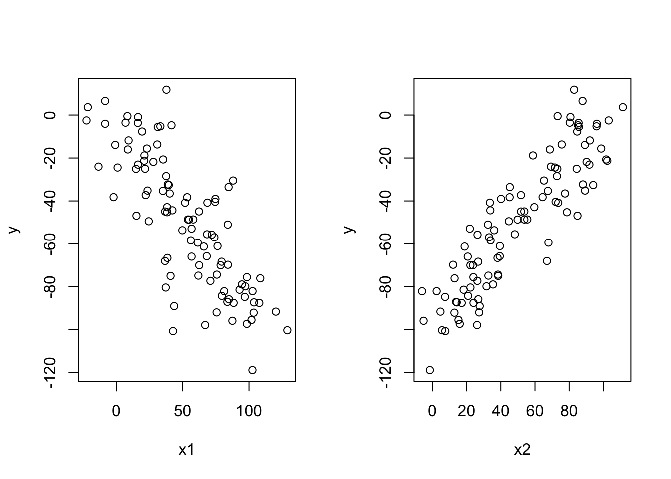
1.16 Correlation coefficient

Question: what is $\rho_{12}$ in left and right figure?

1.17

Correlation coefficient:

$\rho_{12}= \frac{Cov(K_1,K_2)}{\sigma_1\sigma_2}$

Answer to Exercise 5.9:

Start from the definition of $\rho_{12}$ . Compute $Cov(K_1,K_2)$ given that $K_1 = aK_2+b$ ; then use the idea that $Var(K_1) = Var(aK_2+b)$ to find the relation between $\sigma_1$ and $\sigma_2$ .

$$ _{12}= \ Cov(K_1,K_2) = Cov(aK_2+b,K_2) = aCov(K_2,K_2)= aVar(K_2)=a_2^2\ Var(x) = a\ Var(bx) = b^2x\ Var(x+b) = a\ Cov(x,y) = a\ Cov(bx,by) = bba=b^2a\

_1^2 = f(_2^2)\ _1^2 = Var(K_1) = Var(aK_2+b) = a^2Var(K_2) = a^2_2^2\ _1 = |a|2\ {12}== = 1 -1 $$

1.18 Find a portfolio with minimum risk

We are interested in finding a portfolio with minimum risk for any given $\rho_{12}$ such that $-1<\rho_{12}<1$ . We take $s = w_2$ as a parameter:

$\mu_V = w_1\mu_1 + w_2\mu_2$

$s = w_2, w_1+w_2 = 1\\ \begin{aligned} \sigma^2_V&=w_1^2\sigma_1^2+w_2^2\sigma_2^2+2w_1w_2\rho_{12}\sigma_1\sigma_2\\ &=(1-s)^2\sigma_1^2+s^2\sigma_2^2+2(1-s)s\rho_{12}\sigma_1\sigma_2 \end{aligned} \Longrightarrow \sigma_v^2 = f(s)\\ min(f(s)) \rightarrow \frac{\partial f(s)}{\partial s} = 0 \rightarrow s =? \\ \frac{\partial^2 f(s)}{\partial s^2} >0$

1.19

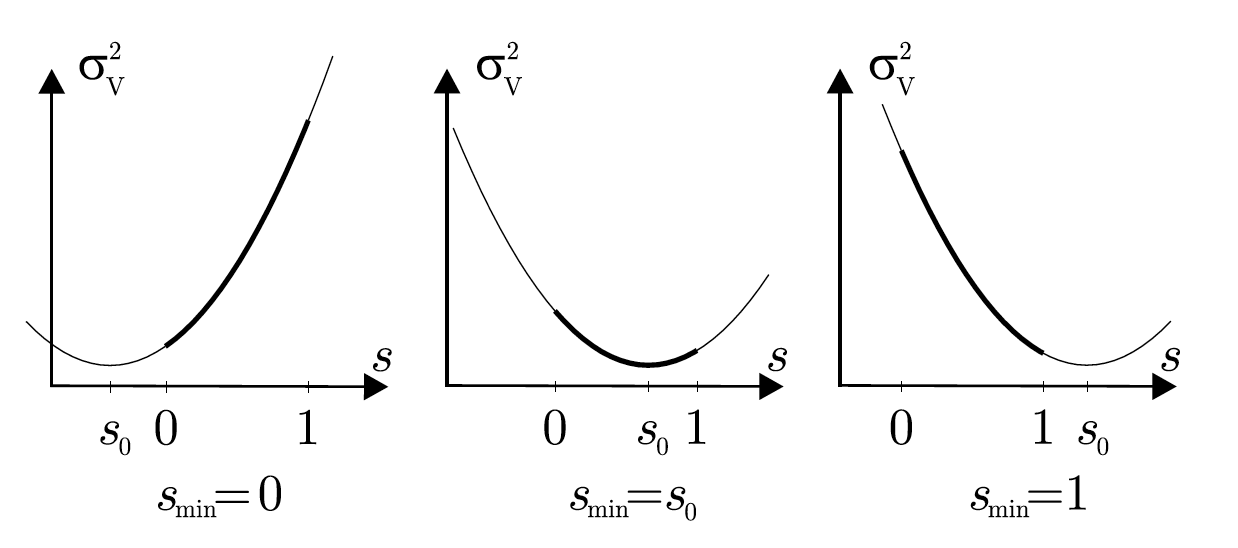
First we find the minimum without any restrictions on short sales.

If short sales are not allowed, we shall have to take into account the bounds $0\leq s\leq 1$ on the parameter.

Theorem For $-1<\rho_{12}<1$ the portfolio with minimum variance is attained at

$s_0 = \frac{\sigma_1^2-\rho_{12}\sigma_1\sigma_2}{\sigma_1^2+\sigma_2^2-2\rho_{12}\sigma_1\sigma_2}$

If short sales are not allowed, then the smallest variance is attained at

$s_{min} =\begin{cases} 0 &\text{if } s_0<0\\ s_0 &\text{if } 0\leq s_0\leq 1\\ 1 &\text{if }1< s_0 \end{cases}$

1.20 Proof

Idea: compute the derivative of $\sigma^2_V$ with respect to $s$ and equate it to 0.

$(1-s)^2\sigma_1^2+s^2\sigma_2^2+2(1-s)s\rho_{12}\sigma_1\sigma_2 = 0\\ \Longrightarrow s = \frac{\sigma_1^2-\rho_{12}\sigma_1\sigma_2}{\sigma_1^2+\sigma_2^2-2\rho_{12}\sigma_1\sigma_2}$

1.21 1.22 Exercise 5.10

Compute the weights in the portfolio with minimum risk for the data in Example 5.6. Does this portfolio involve short selling?

Scenario	Prob.	Return K1	Return K2
w1	0.4	-10%	20%
w2	0.2	0%	20%
w3	0.4	20%	10%

$\sigma_1 = 0.0184, \sigma_2 = 0.0024, \rho_{12}=-0.96309$

1.23

sigma1 = 0.0184
sigma2 = 0.0024
rho12 = -0.96309
s0 = (sigma1^2-rho12*sigma1*sigma2)/(sigma1^2+sigma2^2-2*rho12*sigma1*sigma2)
s0

## [1] 0.8875354

Recitation 5 Note