Chapter 3 Chi-square Goodness of Fit Test
3.1 What is P-value?
In statistics, the p-value is the probability of obtaining results at least as extreme as the observed results of a statistical hypothesis test, assuming that the null hypothesis is correct. The p-value is used as an alternative to rejection points to provide the smallest level of significance at which the null hypothesis would be rejected. A smaller p-value means that there is stronger evidence in favor of the alternative hypothesis.
3.1.1 How Is P-Value Calculated?
P-values are usually found using p-value tables or spreadsheets/statistical software. These calculations are based on the assumed or known probability distribution of the specific statistic being tested. P-values are calculated from the deviation between the observed value and a chosen reference value, given the probability distribution of the statistic, with a greater difference between the two values corresponding to a lower p-value.
Mathematically, the p-value is calculated using integral calculus from the area under the probability distribution curve for all values of statistics that are at least as far from the reference value as the observed value is, relative to the total area under the probability distribution curve. In a nutshell, the greater the difference between two observed values, the less likely it is that the difference is due to simple random chance, and this is reflected by a lower p-value.
3.2 Introduction
A chi-squared test can be used to test the hypothesis that observed data follow a particular distribution. The test procedure consists of arranging the \(n\) observations in the sample into a frequency table with \(k\) classes. For example, suppose for each class, it has a corresponding probability \(p_i\). Then the estimated sequence for all \(k\) classes can be written as \(\{\hat{p}_1,\dots,\hat{p}_k\}\). We want to test the hypothesis
\[ H_0: p_1 = \hat{p}_1, \dots, p_k = \hat{p}_k\\ H_a: o.w. \]
The chi-squared statistic is:
\[ \chi^2 = \sum_{i=1}^{k}\frac{(O_i-E_i)^2}{E_i} \]
where \(O\) is the observed frequency and \(E\) is the expected frequency in each of the response categories. The number of degrees of freedom is \(k − 1\).
3.3 Example: The Poisson Distribution
Let \(X\) be the number of defects in printed circuit boards. A random sample of \(n = 60\) printed circuit boards is taken and the number of defects recorded. The results were as follows:
| Number of defects | Observed Frequency |
|---|---|
| 0 | 31 |
| 1 | 15 |
| 2 | 9 |
| 3 | 4 |
We want to test: Does the assumption of a Poisson distribution seem appropriate as a model for these data?
The null hypothesis is \(H_0 : X\sim Poisson\) The alternative hypothesis is \(H_1 : X\) does not follow a Poisson distribution.
The mean of the (assumed) Poisson distribution is unknown so must be estimated from the data by the sample mean:
\[ \hat{\mu} =\left((32\times0) + (15 \times 1) + (9\times 2) + (4\times3)\right)/60 = 0.75 \]
Using the Poisson distribution with \(\mu = 0.75\) we can compute \(p_i\), the hypothesised probabilities associated with each class. From these we can calculate the expected frequencies (under the null hypothesis):
\[ p_0 = P(X =0) = \frac{e^{-0.75}(0.75)^0}{0!} = 0.472 \Rightarrow E_0 = 0.472\times 60 = 28.32\\ p_1 = P(X =1) = \frac{e^{-0.75}(0.75)^1}{1!} = 0.354 \Rightarrow E_1 = 0.354\times 60 = 21.24\\ p_2 = P(X =2) = \frac{e^{-0.75}(0.75)^2}{2!} = 0.133 \Rightarrow E_2 = 0.133\times 60 = 7.98\\ p_3 = 1 - p_0-p_1-p_2 = 0.041 \Rightarrow E_3 = 0.041\times 60 = 2.46 \]
Note: The chi-squared goodness of fit test is not valid if the expected frequencies are too small. There is no general agreement on the minimum expected frequency allowed, but values of 3, 4, or 5 are often used. If an expected frequency is too small, two or more classes can be combined. In the above example the expected frequency in the last class is less than 3, so we should combine the last two classes to get:
| Number of defects | Observed Frequency |
|---|---|
| 0 | 31 |
| 1 | 15 |
| 2 or more | 13 |
The chi-squared statistic can now be calculated:
\[ \chi^2 =\sum_{i=1}^{k}\frac{(O_i-E_i)^2}{E_i} = \frac{(32-28.32)^2}{28.32} +\frac{(15-21.24)^2}{21.24} + \frac{(13-10.44)^2}{10.44} =2.94 \]
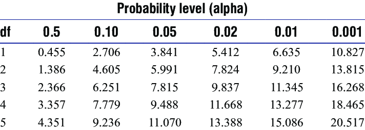
The number of degrees of freedom is \(k − 1\). Here we have \(k = 3\) classes, hence our chi-squared statistic has \(3 − 1 = 2\) degree of freedom (df). If we look up \(2.94\) in tables of the chi-squared distribution with df = 1, we obtain a p-value of \(0.1 < p < 0.5\). We conclude that there is no real evidence to suggest the the data DO NOT follow a Poisson distribution.
3.4 Goodness of fit test for other distributions
The chi-squared goodness of fit test can be used for any distribution. For a discrete distribution the procedure is as described above. For a continuous distribution it is necessary to group the data into classes. Common practice used to carry out the goodness of fit test is to choose class boundaries so that the expected frequencies are equal for each class. For example, suppose we decide to use \(k = 8\) classes. For the standard normal distribution the intervals that divide the distribution into 8 equally likely segments are \([0, 0.32), [0.32, 0.675), [0.675, 1.15), [1.15, \infty)\) and their four “mirror image” intervals below zero. For each interval \(p_i = 1/8\) so the expected frequencies would be \(E_i = n/8\).
3.5 R Example
library(tidyverse) # for ggplot2## ── Attaching packages ─────────────────────────────────────── tidyverse 1.3.1 ──## ✓ ggplot2 3.3.5 ✓ purrr 0.3.4
## ✓ tibble 3.1.2 ✓ dplyr 1.0.7
## ✓ tidyr 1.1.3 ✓ stringr 1.4.0
## ✓ readr 1.4.0 ✓ forcats 0.5.1## ── Conflicts ────────────────────────────────────────── tidyverse_conflicts() ──
## x dplyr::filter() masks stats::filter()
## x dplyr::lag() masks stats::lag()library(magrittr) # for pipes and %<>%##
## Attaching package: 'magrittr'## The following object is masked from 'package:purrr':
##
## set_names## The following object is masked from 'package:tidyr':
##
## extractlibrary(ggpubr)
set.seed(1)
samplesize0=1000
mu0=50
sigma0=10
# 1.1 Index plot of Normal Sample ----
x0<-rnorm(samplesize0,mean=mu0,sd=sigma0)
x <- sort(x0)
# Compute probability integral transform
y=pnorm(x, mean=50, sd=10)
# Set nclass0 (below the chisq gof tests use this variable)
nclass0=20
x.mu<-mu0
x.sigma=sigma0
# Begin True Fit Analysis
hist.1<-hist(100.*pnorm(x,mean=x.mu, sd=x.sigma),
nclass=nclass0,xlab="True Percentile",
main=paste(c("Histogram: True Percentiles\n",
"Normal(mu0, sd0) Distribution\n",
"(N=",as.character(length(y)),")"),collapse=""))
abline(h=length(x)/nclass0, col="green",lwd=2)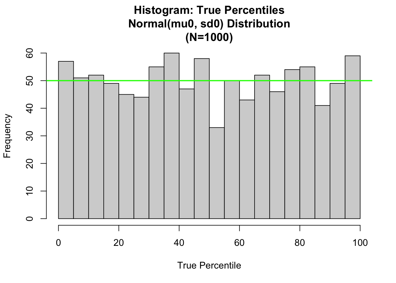
# Compute Chisquare GOF statistic directly
obs.counts<-hist.1$counts
expected.counts<-length(x0)/nclass0
chisq.term<-(obs.counts-expected.counts)^2/expected.counts
df0<-data.frame(k=c(1:length(obs.counts)),Ok=obs.counts,
                Ek=expected.counts,ChiSqk=chisq.term)
print(df0)
## k Ok Ek ChiSqk
## 1 1 57 50 0.98
## 2 2 51 50 0.02
## 3 3 52 50 0.08
## 4 4 49 50 0.02
## 5 5 45 50 0.50
## 6 6 44 50 0.72
## 7 7 55 50 0.50
## 8 8 60 50 2.00
## 9 9 47 50 0.18
## 10 10 58 50 1.28
## 11 11 33 50 5.78
## 12 12 50 50 0.00
## 13 13 43 50 0.98
## 14 14 52 50 0.08
## 15 15 46 50 0.32
## 16 16 54 50 0.32
## 17 17 55 50 0.50
## 18 18 41 50 1.62
## 19 19 49 50 0.02
## 20 20 59 50 1.62print(sum(df0$ChiSqk))## [1] 17.52In R, the function chisq:test() implements the chi-square goodness of fit test.
# Apply function chisq.test to obs.counts
chisq.test.1<-chisq.test(obs.counts, correct=FALSE)
print(chisq.test.1)
##
## Chi-squared test for given probabilities
##
## data: obs.counts
## X-squared = 17.52, df = 19, p-value = 0.5547chisq.test.1$residuals## [1] 0.9899495 0.1414214 0.2828427 -0.1414214 -0.7071068 -0.8485281
## [7] 0.7071068 1.4142136 -0.4242641 1.1313708 -2.4041631 0.0000000
## [13] -0.9899495 0.2828427 -0.5656854 0.5656854 0.7071068 -1.2727922
## [19] -0.1414214 1.2727922pval<-formatC(chisq.test.1$p.value,format = "e", digits = 2)
main.title<-paste(c("Chisquare Residuals","\n Chi-Square Stat = ",
as.character(round(chisq.test.1$statistic),digits=2),
" (P-Value = ", pval,")"), collapse="")
barplot(chisq.test.1$residuals)
title(main=main.title)
# expected level of residuals
exp.level=1.1
abline(h=c(1,-1)*exp.level,col="green")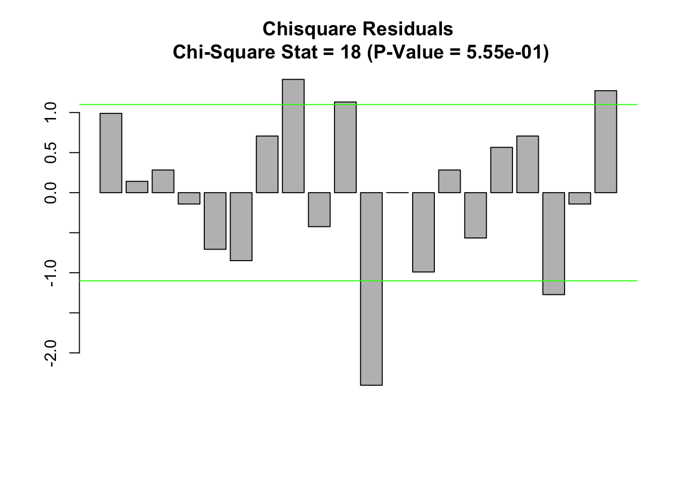
# Set nclass0 (below the chisq gof tests use this variable)
nclass0=20
x.mu.robust<-median(x)
x.sigma.robust<-IQR(x)/1.3490
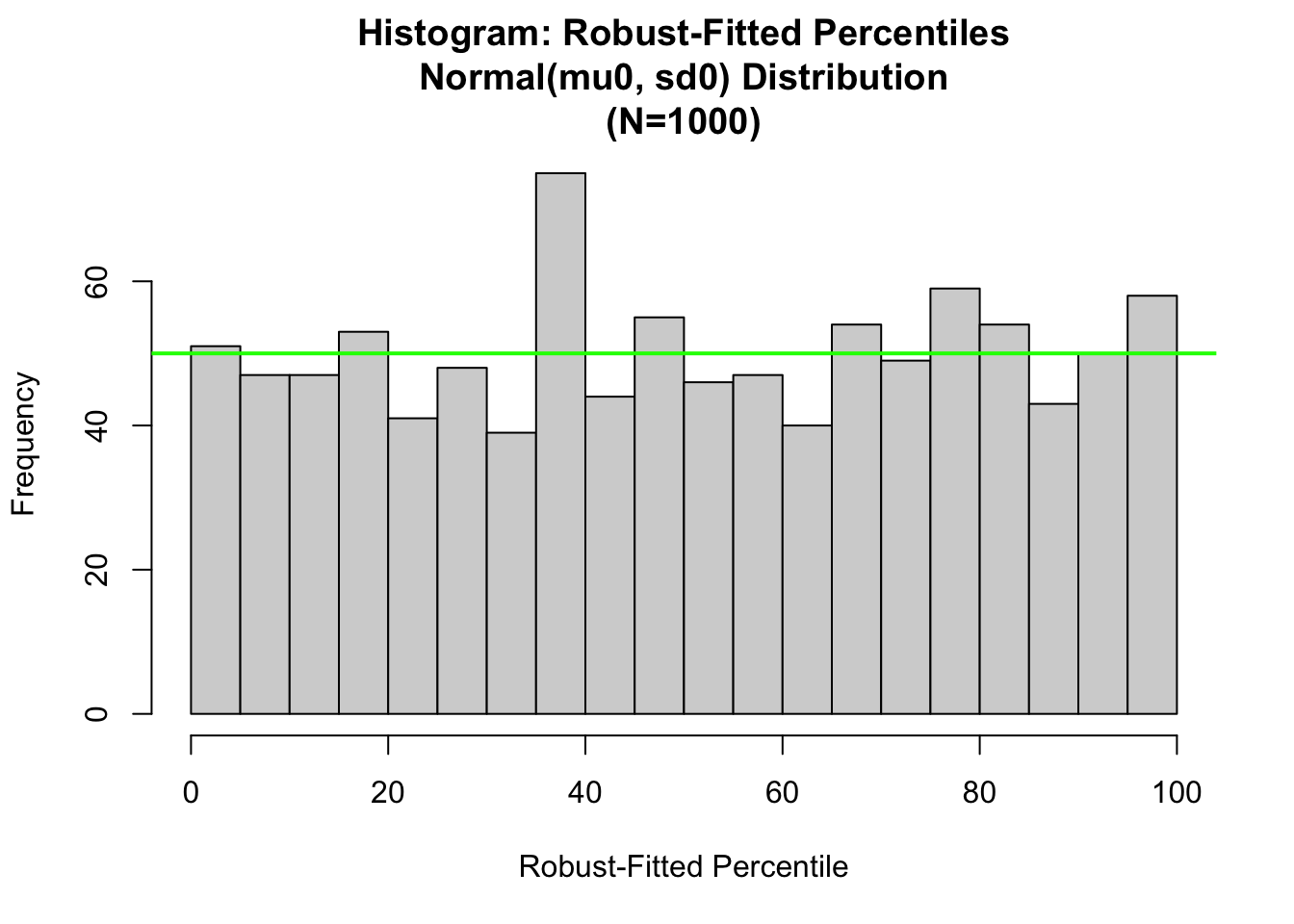
# Begin Robust Fit Analysis
hist.1<-hist(100.*pnorm(x,mean=x.mu.robust, sd=x.sigma.robust),
nclass=nclass0,xlab="Robust-Fitted Percentile",
main=paste(c("Histogram: Robust-Fitted Percentiles\n",
"Normal(mu0, sd0) Distribution\n",
"(N=",as.character(length(y)),")"),
collapse=""))
abline(h=length(x)/nclass0, col="green",lwd=2)