Chapter 1 Goodness of Fit

1.1 Probability Model for Asset Returns

Consider a data set of daily asset percent returns:

\[ x_1, x2,\dots, x_n \]

Assume the return on day \(t\) is a random variable \(X_t\):

The set of all possible outcomes of \(X_t = x_t\) is the set of real numbers

\[ \{\text{all possible }X_t\} =\{-\infty <x_t<\infty\} \]

The probability model/distribution for \(X_t\) is given by specifying the cumulative distribution function or equivalently the probability density function
Special Cases of the Probability Model in our exercise
- Case 1: Normal Model. If \(X_t\sim Normal(\mu,\sigma)\) then
\[ f(x_t) = \frac{1}{\sqrt{2\pi}\sigma}e^{-\frac{1}{2}\frac{(x-\mu)^2}{\sigma^2}} \]
- Case 2: Laplace Model. If \(X_t\sim Laplace(\mu,b)\) then
\[ f(x) = \frac{1}{2b}e^{-\frac{|x-\mu|}{b}} \]

1.2 Fitting Probability Models

Useful methods for estimating the parameters of a probability model are the Method-of-Moments and Maximum Likelihood.

1.2.1 Maximum Likelihood Estimation

1.2.1.1 Introduction

The Maximum Likelihood Estimation (MLE) is a method of estimating the parameters of a model. This estimation method is one of the most widely used.
The method of maximum likelihood selects the set of values of the model parameters that maximizes the likelihood function. Intuitively, this maximizes the “agreement” of the selected model with the observed data.
The Maximum-likelihood Estimation gives an uniÖed approach to estimation.

1.2.1.2 The Principle of Maximum Likelihood

We take poisson distributed random variables as an example. Suppose that \(X_1,X_2,\dots,X_N\) are i.i.d. discrete random variables, such that \(Xi\sim Pois(\theta)\) with a pmf (probability mass function) defined as:

\[ Pr(X_i = x_i) = \frac{\exp(-\theta)\theta^{x_i}}{x_i!} \]

where \(\theta\) is an unknown parameter to estimate.

Question: What is the probability of observing the particular sample \(\{x_1, x_2,\dots, x_N\}\), assuming that a Poisson distribution with as yet unknown parameter \(\theta\) generated the data?

This probability is equal to

\[ Pr((X_1 = x_1)\cap\dots\cap (X_N = x_N )) \]

Since the variables \(X_i\) are i.i.d., this joint probability is equal to the product of the marginal probabilities:

\[ Pr((X_1 = x_1)\cap\dots\cap (X_N = x_N )) = \prod_{i=1}^N Pr(X_i = x_i) \]

Given the pmf of the Poisson distribution, we have:

\[ Pr((X_1 = x_1)\cap\dots\cap (X_N = x_N )) = \prod_{i=1}^N \frac{\exp(-\theta)\theta^{x_i}}{x_i!} = \exp(-\theta N)\frac{\theta^{\sum_{i=1}^N x_i}}{\prod_{i=1}^N x_i !} \]

This joint probability is a function of \(\theta\) (the unknown parameter) and corresponds to the likelihood of the sample \(\{x_1, x_2,\dots, x_N\}\) denoted by

\[ \mathcal{L}(x_1,\dots,x_N|\theta) = Pr((X_1 = x_1)\cap\dots\cap (X_N = x_N )) \]

Consider maximizing the likelihood function \(\mathcal{L}(x_1,\dots,x_N|\theta)\) with respect to \(\theta\). Since the log function is monotonically increasing, we usually maximize \(\ln \mathcal{L}(x_1,\dots,x_N|\theta)\) instead. We call this as loglikelihood function: \(\ell(x_1,\dots,x_N|\theta) = \ln \mathcal{L}(x_1,\dots,x_N|\theta)\), or simply \(\ell(\theta)\). In this case:

\[ \ell (x_1,\dots,x_N|\theta) = -\theta N + \ln(\theta)\sum_{i=1}^N x_i - \ln(\prod_{i=1}^N x_i !) \]

The simplest way to find the \(\theta\) that maximizes \(\ell(\theta)\) is to take a derivative.

\[ \frac{\partial\ell(\theta)}{\partial \theta} = -N + \frac{1}{\theta}\sum_{i=1}^N x_i \]

To make sure that we indeed maximize not minimize \(\ell(\theta)\), we should also check that the second derivative is less than 0:

\[ \frac{\partial^2\ell(\theta)}{\partial \theta^2} = - \frac{1}{\theta^2}\sum_{i=1}^N x_i < 0 \]

Therefore, the maximum likelihood estimator \(\hat{\theta}_{mle}\) is:

\[ \hat{\theta}_{mle} = \frac{1}{N}\sum_{i=1}^N x_i \]

For the Laplace model, the maximum-likelihood estimates are:

\[ \hat{\mu} = median(x_t)\\ \hat{b} = \frac{1}{n}\sum_{i=1}^n|x_t-\hat{\mu}| \]

Note that they are different from the MOM results.

1.3 Chi-Square Goodness-of-Fit Test for True Model

The Chi-Square Goodness-of-Fit (GOF) Test applies to evaluating whether sample data is consistent with coming from a given probability distribution. The evaluation compares the empirical histogram of the sample data to the theoretical histogram of the given probability distribution.

Suppose \(X_1,\dots,X_n\)is a random sample from the probability distribution with cumulative distribution function \(F\):

Then, the percentiles \(Y_1,\dots,Y_n\) where \(Y_i = F(X_i)\) are random variables which are an i.i.d. sample from the \(Uniform(0,1)\) distribution.

We simulated a sample from the \(Normal(\mu_0,\sigma_0)\) distribution with mean \(\mu_0 = 50\) and standard deviation \(\sigma_0 = 10\). We use R to compute the realized percentiles and evaluate the goodness of fit test for whether these are consistent with being a random sample from the \(Uniform(0,1)\) distribution.

library(tidyverse) # for ggplot2

## ── Attaching packages ─────────────────────────────────────── tidyverse 1.3.1 ──

## ✓ ggplot2 3.3.5     ✓ purrr   0.3.4
## ✓ tibble  3.1.2     ✓ dplyr   1.0.7
## ✓ tidyr   1.1.3     ✓ stringr 1.4.0
## ✓ readr   1.4.0     ✓ forcats 0.5.1

## ── Conflicts ────────────────────────────────────────── tidyverse_conflicts() ──
## x dplyr::filter() masks stats::filter()
## x dplyr::lag()    masks stats::lag()

library(magrittr) # for pipes and %<>%

## 
## Attaching package: 'magrittr'

## The following object is masked from 'package:purrr':
## 
##     set_names

## The following object is masked from 'package:tidyr':
## 
##     extract

library(ggpubr)

set.seed(1)
samplesize0=1000
mu0=50
sigma0=10
# 1.1 Index plot of Normal Sample ----
x0<-rnorm(samplesize0,mean=mu0,sd=sigma0)
x <- sort(x0)

# Compute probability integral transform
# y0<-pnorm(x0, mean=mu0, sd=sigma0)
y=pnorm(x, mean=50, sd=10)
# Set nclass0 (below the chisq gof tests use this variable)
nclass0=20
x.mu<-mu0
x.sigma=sigma0
# Begin True Fit Analysis
hist.1<-hist(100.*pnorm(x,mean=x.mu, sd=x.sigma),
              nclass=nclass0,xlab="True Percentile",
              main=paste(c("Histogram: True Percentiles\n",
                        "Normal(mu0, sd0) Distribution\n",
                        "(N=",as.character(length(y)),")"),collapse=""))
abline(h=length(x)/nclass0, col="green",lwd=2)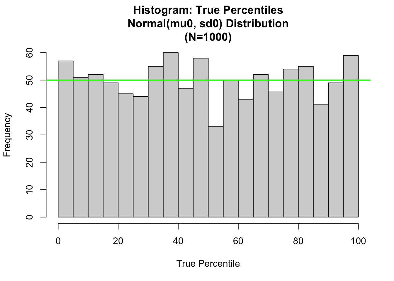

For convenience, we have rescaled the percentiles from the (0,1) scale to (0,100) scale. The theoretical histogram for the True Percentiles is the uniform distribution. With \(N = 1000\); and nclass0 = 20; the number of bins, we expect there to be \(E = N/nclass0 = 50\) sample values in each bin. This is displayed as the green level in the plot.

Lecture 6 Note