Chapter 2 Maximum Likelihood Estimation
2.1 A quick review on different distributions
x <- seq(-12, 12, length=10000)
ynorm1 <- dnorm(x, mean=0, sd=1)
ynorm2 <- dnorm(x, mean=0, sd=2)
ynorm3 <- dnorm(x, mean=0, sd=4)
ynorm4 <- dnorm(x, mean=2, sd=4)
plot(x, ynorm1, type="l", lwd=1,col = 'blue',
     main = "Normal distribution with different mean and sd")
lines(x, ynorm2, type="l", lwd=1,col = 'red')
lines(x, ynorm3, type="l", lwd=1,col = 'green')
lines(x, ynorm4, type="l", lwd=1,col = 'purple')
legend('topright',legend = c("mean = 0, sd = 1","mean = 0, sd = 2",
                  "mean = 0, sd = 4","mean = 2, sd = 4"),
       col=c("blue", "red", 'green', 'purple'), lty=1, cex=0.8)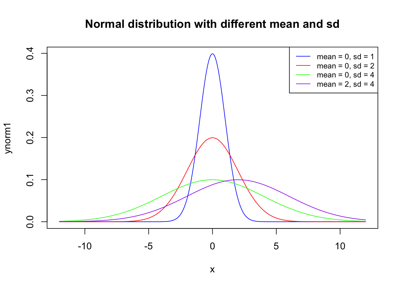
2.1.1 Laplace distribution
The Laplace distribution is a continuous probability distribution. It is also sometimes called the double exponential distribution, because it can be thought of as two exponential distributions (with an additional location parameter) spliced together, back-to-back.
library("VGAM")## Loading required package: stats4## Loading required package: splinesx <- seq(-12, 12, length=10000)
ylap1 <- dlaplace(x, location=0, scale=1)
ylap2 <- dlaplace(x, location=0, scale=2)
ylap3 <- dlaplace(x, location=0, scale=4)
ylap4 <- dlaplace(x, location=2, scale=4)
plot(x, ylap1, type="l", lwd=1,col = 'blue',
main = "Laplace distribution with different location and scale")
lines(x, ylap2, type="l", lwd=1,col = 'red')
lines(x, ylap3, type="l", lwd=1,col = 'green')
lines(x, ylap4, type="l", lwd=1,col = 'purple')
legend('topright',legend = c("location = 0, scale = 1","location = 0, scale = 2",
"location = 0, scale = 4","location = 2, scale = 4"),
col=c("blue", "red", 'green', 'purple'), lty=1, cex=0.8)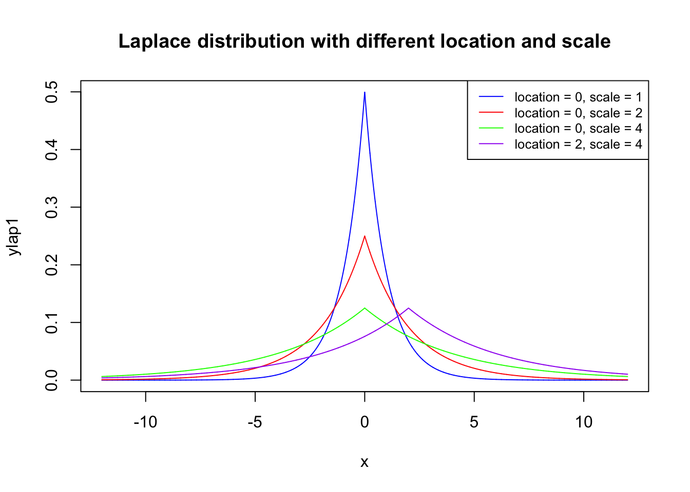
A random variable has a \(Laplace(\mu ,b)\) distribution if its probability density function is
\[ f(x|\mu,b) = \frac{1}{2b}\exp(-\frac{|x-\mu|}{b}) \]
Here, \(\mu\) is a location parameter and \(b > 0\), which is sometimes referred to as the diversity, is a scale parameter. If \(\mu =0\) and \(b=1\), the positive half-line is exactly an exponential distribution scaled by 1/2.
x <- seq(-12, 12, length=10000)
ylap1 <- dlaplace(x, location=0, scale=1)
yexp1 <- dexp(x, rate = 0.5)
plot(x, ylap1, type="l", lwd=1,col = 'blue',ylim=c(0,0.7))
lines(0.5*x, yexp1, type="l", lwd=2,col = 'red')
legend("topright",legend = c("Laplace dist with location = 0 and scale = 1",
                             "Exponential dist with rate = 0.5 and scale by 0.5"),
       col=c('blue','red'),lty=1)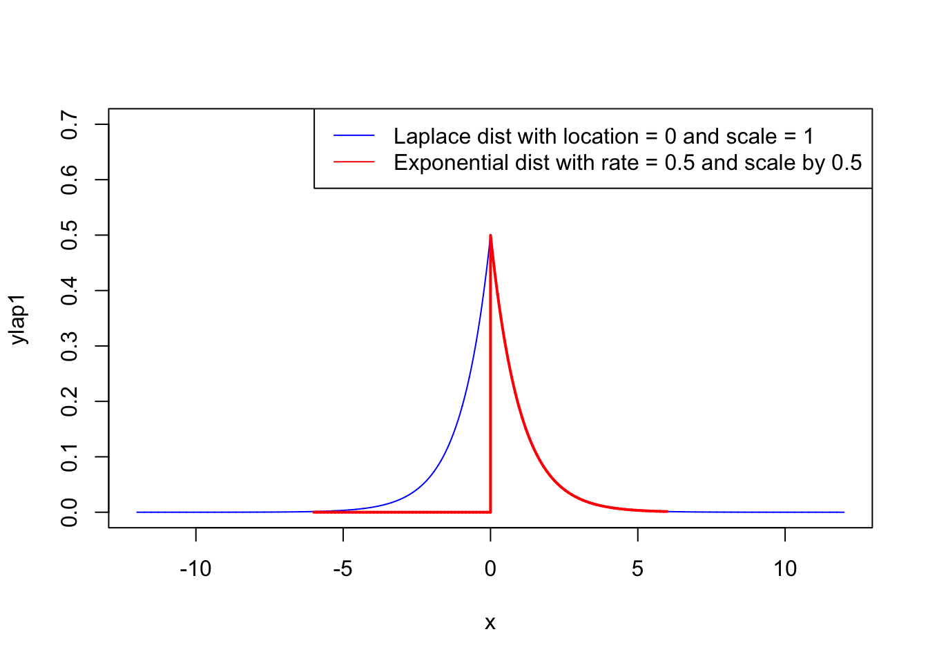
2.2 Introduction
The Maximum Likelihood Estimation (MLE) is a method of estimating the parameters of a model. This estimation method is one of the most widely used.
The method of maximum likelihood selects the set of values of the model parameters that maximizes the likelihood function. Intuitively, this maximizes the “agreement” of the selected model with the observed data.
The Maximum-likelihood Estimation gives an uniÖed approach to estimation.
2.3 The Principle of Maximum Likelihood
We take poisson distributed random variables as an example. Suppose that \(X_1,X_2,\dots,X_N\) are i.i.d. discrete random variables, such that \(Xi\sim Pois(\theta)\) with a pmf (probability mass function) defined as:
\[ Pr(X_i = x_i) = \frac{\exp(-\theta)\theta^{x_i}}{x_i!} \]
where \(\theta\) is an unknown parameter to estimate.
Question: What is the probability of observing the particular sample \(\{x_1, x_2,\dots, x_N\}\), assuming that a Poisson distribution with as yet unknown parameter \(\theta\) generated the data?
This probability is equal to
\[ Pr((X_1 = x_1)\cap\dots\cap (X_N = x_N )) \]
Since the variables \(X_i\) are i.i.d., this joint probability is equal to the product of the marginal probabilities:
\[ Pr((X_1 = x_1)\cap\dots\cap (X_N = x_N )) = \prod_{i=1}^N Pr(X_i = x_i) \]
Given the pmf of the Poisson distribution, we have:
\[ Pr((X_1 = x_1)\cap\dots\cap (X_N = x_N )) = \prod_{i=1}^N \frac{\exp(-\theta)\theta^{x_i}}{x_i!} = \exp(-\theta N)\frac{\theta^{\sum_{i=1}^N x_i}}{\prod_{i=1}^N x_i !} \]
This joint probability is a function of \(\theta\) (the unknown parameter) and corresponds to the likelihood of the sample \(\{x_1, x_2,\dots, x_N\}\) denoted by
\[ \mathcal{L}(x_1,\dots,x_N|\theta) = Pr((X_1 = x_1)\cap\dots\cap (X_N = x_N )) \]
Consider maximizing the likelihood function \(\mathcal{L}(x_1,\dots,x_N|\theta)\) with respect to \(\theta\). Since the log function is monotonically increasing, we usually maximize \(\ln \mathcal{L}(x_1,\dots,x_N|\theta)\) instead. We call this as loglikelihood function: \(\ell(x_1,\dots,x_N|\theta) = \ln \mathcal{L}(x_1,\dots,x_N|\theta)\), or simply \(\ell(\theta)\). In this case:
\[ \ell (x_1,\dots,x_N|\theta) = -\theta N + \ln(\theta)\sum_{i=1}^N x_i - \ln(\prod_{i=1}^N x_i !) \]
The simplest way to find the \(\theta\) that maximizes \(\ell(\theta)\) is to take a derivative.
\[ \frac{\partial\ell(\theta)}{\partial \theta} = -N + \frac{1}{\theta}\sum_{i=1}^N x_i \]
To make sure that we indeed maximize not minimize \(\ell(\theta)\), we should also check that the second derivative is less than 0:
\[ \frac{\partial^2\ell(\theta)}{\partial \theta^2} = - \frac{1}{\theta^2}\sum_{i=1}^N x_i < 0 \]
Therefore, the maximum likelihood estimator \(\hat{\theta}_{mle}\) is:
\[ \hat{\theta}_{mle} = \frac{1}{N}\sum_{i=1}^N x_i \]