Based on the data cleaning, this page explains all plots in Summary, Forest Plot, Intervention Detail, Comparison tabs.
3.1 Summary
3.1.1 Year of Publication
This bar chart tracks the number of studies published over time. It allows users to quickly assess trends in research output and identify potential peaks or declines in study publications within the dataset.
3.1.2 Year of Publication by Selected Variables
This stacked bar chart breaks down publications by year and region, offering insights into the geographical distribution of research over time. It can reveal which regions are contributing more to the field or how research focus shifts geographically.
3.1.3 Intervention Subcode
This bar chart lists various interventions and the count of studies associated with each, giving an overview of the types of interventions investigated and their prevalence in the research.
3.1.4 Outcome Subcode
The pie chart displays the proportion of different outcomes studied, offering a visual summary of the research focus areas within the dataset.
3.1.5 Publication Type
This pie chart shows the distribution of the types of publications (journal articles, reports, conference proceedings, etc.), highlighting the primary sources of research data.
3.1.6 Evaluation Design
Another pie chart presents the various research designs used in the studies, such as randomized controlled trials or statistical matching, providing insight into the methodological approaches in the dataset.
3.1.7 Region
The chart depicts the proportion of studies conducted in different global regions, offering a view of the geographical spread of research efforts.
3.1.8 Income Level
This pie chart categorizes studies according to the income level of the countries or regions they pertain to, which can be vital for understanding the socio-economic contexts of the research.
3.2 Forest Plot
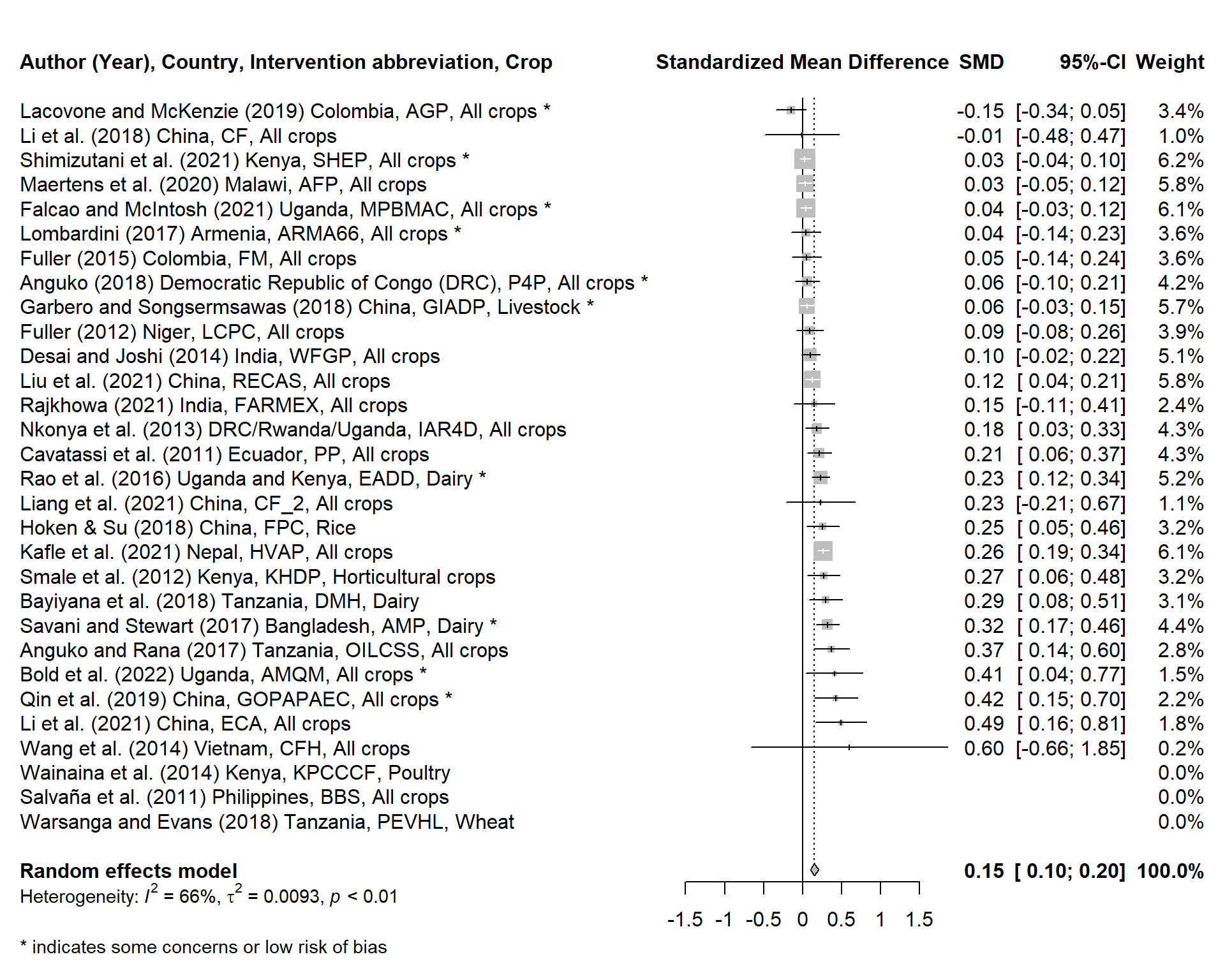
“The most common way to visualize meta-analyses is through forest plots. Such plots provide a graphical display of the observed effect, confidence interval, and usually also the weight of each study. They also display the pooled effect we have calculated in a meta-analysis. Overall, this allows others to quickly examine the precision and spread of the included studies, and how the pooled effect relates to the observed effect sizes.”
— Harrer, M., Cuijpers, P., Furukawa, T.A., & Ebert, D.D. (2021). Doing Meta-Analysis with R: A Hands-On Guide. Boca Raton, FL and London: Chapman & Hall/CRC Press. ISBN 978-0-367-61007-4.
3.2.1 Forest Plot Generator (Control Box)
Display of Missing Effect Sizes: Users can choose whether to include studies with missing effect sizes (NA) in the forest plot.
English Style: The application allows for customization of the forest plot annotations based on English language variations (US or UK), affecting spellings such as “standardized” (US) vs “standardised” (UK).
Risk of Bias Levels: Users can specify the risk of bias level for each study, which may be visually differentiated in the plot, for example with asterisks or color coding.
Regions: The application can filter or group data by specified regions such as Sub-Saharan Africa, East Asia & Pacific, etc., which can be particularly useful in analyses that require regional stratification.
Income Level: Similar to region filtering, users can filter or stratify the data based on income levels, which is useful for socio-economic subgroup analyses.
Model Statistics Display: Users have control over the meta-analysis model type and can choose to display statistics relevant to random effects models, such as the Q statistic, I statistic, and Tau statistic.
3.2.2 Forest Plot Generator
Despite the utilization of different measurement approaches within the meta-analysis, it is noteworthy that the majority of statistical outcomes appear remarkably consistent across the methodologies employed. This observation underscores a fundamental aspect of meta-analytic procedures: while the specific analytic tools and models might vary — for instance, between the metafor and meta packages — the core objective remains the robust estimation and interpretation of effect sizes across a body of research. For the graphical purpose, the forest plot will be based on metagen from meta package.
Metric
Metafor Statistics
Meta Statistics
Difference
Number of estimations
27.000
27.000
No
Tau Squared (tau^2)
0.009
0.009
No
Tau (tau)
0.097
0.097
No
I Squared (I^2)
66.196
66.196
No
H Squared (H^2)
2.958
2.958
No
Test for Heterogeneity: Q
76.913
76.913
No
Degrees of Freedom (df)
26.000
26.000
No
p-value of Q
0.000
0.000
No
Effect Size
0.152
0.152
No
Standard Error (se)
0.026
0.026
No
z-value
5.943
5.943
No
p-value
0.000
0.000
No
CI Lower Bound
0.102
0.102
<0.001
CI Upper Bound
0.202
0.202
No
Statistics differences
3.2.3 Plot output
The forest plot, a quintessential tool in meta-analysis for visualizing study effects and confidence intervals, is generated through the forest.meta function.
resoutcomesubcode_meta <-metagen(TE = yi, seTE =sqrt(vi), data = current_data, sm ="SMD",fixed = F,random = T,method.tau ="DL",studlab = authors_ctry_rob_inter)forest.meta(resoutcomesubcode_meta,sortvar = TE,leftcols =c("studlab"),leftlabs =c("Author (Year), Country, Intervention abbreviation, Crop "),weight.study ="common",digits.TE =2,smlab ="Standardized Mean Difference", # This commend specifies the display option whether Us or UK English sytle.text.addline2 =format("\n\n* indicates some concerns or low risk of bias"))
3.3 Intervention Detail
3.3.1 Geographical Frequency in Continent or Country Level
This interactive world map is color-coded to indicate the frequency of studies across continents and countries. It allows users to easily pinpoint the most researched areas in agricultural studies, adaptable to continent and country selections for focused analysis.
3.3.2 The Most Frequent Words in Intervention Description
A dynamic word cloud presents the most common terms used in intervention descriptions. The word size reflects usage frequency, aiding in the quick identification of predominant themes. The text is processed for stemming to ensure similar terms are consolidated for accurate representation.
3.3.3 Intervention Summary
This section provides a comprehensive list of intervention types, their subcodes, definitions, and the count of studies that investigated them. It serves to inform users about the most common intervention strategies and their distribution across the research landscape.
3.3.4 Intervention Description in the Extracted Coding
This area allows for the selection of an intervention subcode to view detailed descriptions and definitions. It also lists the studies that have included the selected intervention, providing a deeper understanding of the context and application of each intervention type.
3.3.4.1Confidence Interval and Effect Size Plot
A plot that displays the effect size of selected studies with their corresponding confidence intervals. The presence of the effect size on either side of the zero line indicates the direction of the effect, and the span of the confidence interval indicates the precision of the estimate.
3.4 Comparison
In the application, a specialized tab facilitates comparative analysis under two distinct scenarios: “Risk of Bias” and “Outliers.” Users can choose one scenario to shape their analysis:
Risk of Bias: When this option is selected, the application compares the effect estimates of the full studies against a subset where high-risk studies are excluded (only some concerns and low risk of bias).
Outliers: By choosing this option, the application contrasts the effect estimates from all studies with those from a dataset where outliers are omitted, illuminating how these extreme values might skew the overall findings.
3.4.1 Boxplot
This plot will categorize studies according to the selected input and display their effect sizes. It’s a visual tool to quickly discern the spread and central tendency of effects within each category.
3.4.2 Study Level Estimates
Following the boxplot, detailed plots show individual study estimates alongside their confidence intervals. This visual representation helps to pinpoint the precise effect each study contributes to the overall analysis.
3.4.3 Comparative Analysis Plot
At the bottom, a plot compares the average effects and confidence intervals of all studies against those after excluding either high-risk studies or outliers. This comparison illustrates how the inclusion or exclusion of certain studies can influence the meta-analysis results.
3.5 Takeaways
Data Visualization: Insightful visuals track publication trends and regional distribution, offering a snapshot of the research landscape over time and by location.
Intervention Detail: Detailed breakdowns of intervention strategies and outcomes, with interactive maps and word clouds for in-depth analysis.
Forest Plot: A key graphical representation of individual and pooled study effects, essential for a quick assessment of research findings.
Comparison: A focused comparison of studies considering the risk of bias and outliers, highlighting the impact of these factors on the meta-analysis.