Chapter 10 Multiple OLS Regression
This chapter provides generic code for carrying out a multiple OLS regression analysis. It is recommended that you proceed through the sections in the order they appear.
10.1 Packages Needed for Multiple OLS Regression
This code will check that required packages for this chapter are installed, install them if needed, and load them into your session.
req <- substitute(require(x, character.only = TRUE))
libs<-c("sjPlot", "stargazer", "coefplot", "dotwhisker", "visreg", "jtools", "ggfortify", "olsrr", "DescTools", "interactions")
sapply(libs, function(x) eval(req) || {install.packages(x); eval(req)})
10.2 Data Prep for Multiple OLS Regression
One of the key preparations you need to make is to declare (classify) your categorical variables as factor variables. In the generic commands below, the ‘class’ function tells you how R currently sees the variable (e.g., double, factor, character). The second command will reclassify the specified categorical variable as a factor variable.
class(mydata$var)
mydata$catvar <- factor(mydata$catvar)
You can also change the reference group on a factor variable (specify the desired level, as it is not determined by assigned numbers). By default, the first category will serve as the reference group in categorical variables included as independent variables.
mydata$catvar <- relevel(mydata$catvar, ref = #)10.3 Basic OLS Regression Commands
object <- lm(depvar ~ indvar1 + indvar2 + indvar3, data = mydata)
summary(object)
10.4 Diagnostic Plots for Multiple OLS Regression
There are a few different packages that are useful for producing diagnostic plots or related statistics: ggplot’s autoplot (enabled by ggfortify) (for multiple diagnostics at once using the autoplot function); DescTools::VIF; and olsrr’s various functions (for various individual diagnostics)
ggplot2::autoplot(object, which = 1:6, ncol = 2)

DescTools::VIF(object) # Multicollinearity test (VIFs)

olsrr::ols_coll_diag(object) # Multicollinearity test (VIFs)
olsrr::ols_test_breusch_pagan(object) # Test of Homo/Heteroskedasticity
olsrr::ols_plot_dfbetas(object)  # Influential observations
olsrr::ols_plot_cooksd_bar(object)  # Influential observations
olsrr::ols_plot_cooksd_chart(object)   # Influential observations
olsrr:ols_plot_resid_stand(object)   # Influential observations
olsrr::ols_plot_resid_lev(object)   # Influential observations
olsrr::ols_plot_resid_pot(object)   # Influential observations
10.5 Outliers - Identifying and Excluding
Since outliers may be biasing estimates, you may want to exclude them from the sample in order to see how the model changes in their absence (i.e., improved fit; changes in coefficients). This series of commands accomplishes this task. In the commands, be sure to substitute the actual sample size for “N.”
object <- lm(depvar ~ indvar1 + indvar2, data = mydata)
jtools::summ(object)   # To get the N of the model
4/N   # So you know a traditional cut-off point for identifying outliers
cooksd <- cooks.distance(object)
influential <- as.numeric(names(cooksd)[(cooksd > (4/N))])

# Or

influential <- as.numeric(names(cooksd)[(cooksd > #)])   # Replace # with the desired cut-off value
mydata_noout <- mydata[-influential, ]   # This will create a second data set absent the outliers
10.6 Producing Formatted Tables of Multiple OLS Regression Results
sjPlot’s tab_model function works really well for producing formatted tables, especially if you only have one to three models. You can find helpful insights on sjPlot’s tab_model function here. The stargazer package/function also produces nicely formatted html tables (saved to your working directory) that can be copied/pasted into Word.
sjPlot::tab_model(object)

sjPlot::tab_model(object1, object2, pred.labels = c("Intercept", "iv1 label", "iv2 label"),
  dv.labels = c("Model 1", "Model 2"), string.pred = "Estimates", string.ci = "95% CIs",
  string.p = "p-values")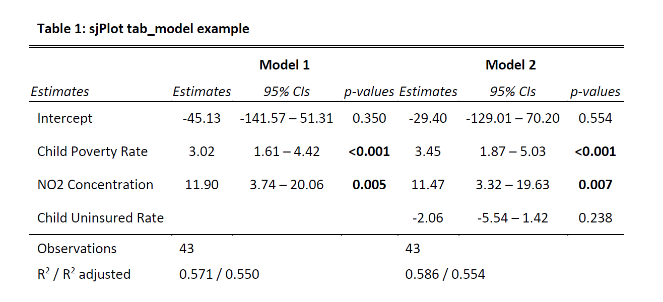
The stargazer package/function offers another alternative for generating formatted tables.
stargazer(object1, object2, type = "html", ci = TRUE, digits = 2, ci.separator = "-",
  star.cutoffs = c(.05, .01, .001), title = "Title of Table", covariate.labels =
  c("indvar1 label", "indvar2 label", "indvar3 label", "Intercept"),
  dep.var.labels = c("depvar label"), out = "filename.htm")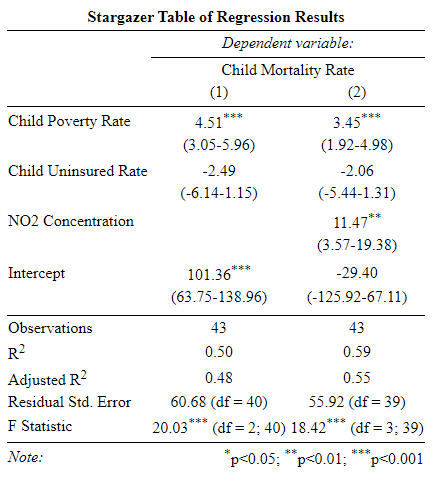
10.7 Graphing Coefficients and CIs for Multiple OLS Regression
It is often helpful to graphically represent regression coefficients and their CIs. The sjPlot, dotwhisker, and coefplot packages all offer options in this regard.
Note: These commands make use of the “object”(s) generated by your regression commands.
sjPlot::plot_model(object, show.values = TRUE)When plotting more than one model with sjPlot, I find that I prefer to switch the order of my objects.
sjPlot::plot_models(object2, object1, show.values = TRUE, show.legend = FALSE)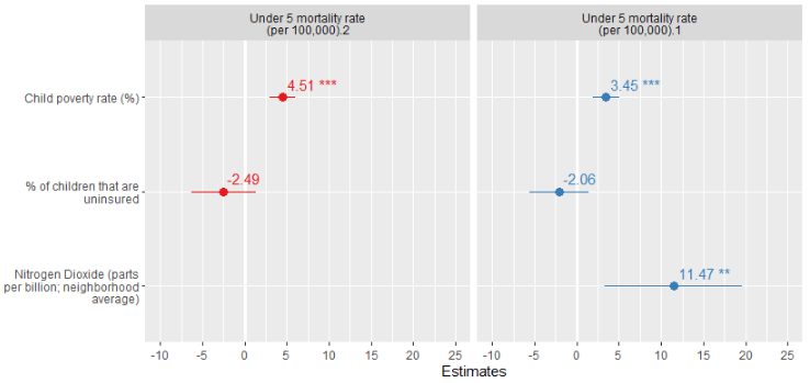
The following two functions offer additional options for plotting regression results, though I find them less appealing than sjPlot’s plot_model(s) functions.
dotwhisker::dwplot(object)
coefplot::coefplot(object)
jtool’s plot_summs function is yet another option. These commands can be used following the generation of your model(s) (i.e., object(s)):
jtools::plot_summs(object, scale = TRUE, plot.distributions = TRUE, inner_ci_level = .9)
jtools::plot_summs(object, object2, scale = TRUE)
jtools::plot_summs(object, object2, scale = TRUE, plot.distributions = TRUE,
  coefs = c("Desired Variable Name" = "var1", "Desired Variable Name" = "var2"))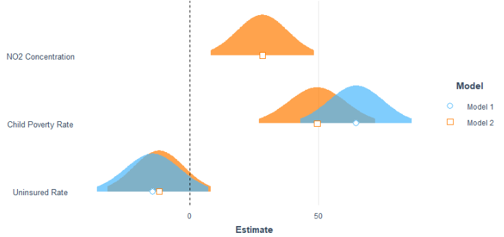
10.8 Graphing Margins (Predicted Values) for Multiple OLS Regression
In addition to graphing regression coefficients and their CIs, it can often be helpful to calculate and graph marings or predicted values of Y at different values of X. I’m partial to the visreg package/function, though jtool’s effect_plot is another option.
visreg(object, "var", ylab = "Y-axis label", xlab = "X-axis label")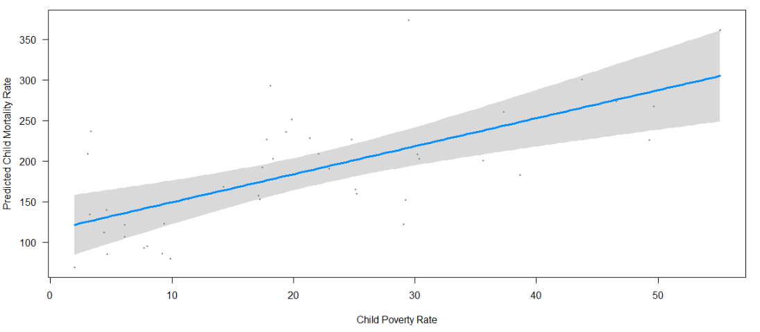
jtools::effect_plot(object, pred = iv1, interval = TRUE, y.label = "label", x.label = "label")10.9 Modeling and Graphing Interactions for Multiple OLS Regression
Modeling and interpreting interactions from regression coefficients alone can be difficult. Graphing the results is helpful in this regard. Both the interactions package and sjPlot offer assistance in this regard. Both show the predicted value of Y based on the interaction of the specified predictors.
object <- lm(depvar ~ intvar * catvar, data = mydata)
summary(object)
interactions::interact_plot(object, pred = intvar, modx = catvar)

# sjPlot’s version

object <- lm(depvar ~ intvar * catvar, data = mydata)
sjPlot::plot_model(object, type = "pred", terms = c("intvar", "catvar"))
10.10 Consolidated Code for Multiple OLS Regression
Below is the consolidated code from this chapter. One could transfer this code into an empty RScript, which also offers the option of find/replace terms. You can also download this generic Multiple OLS Regression RScript file here.
Placeholders that need replacing:
- mydata – name of your dataset
- var – general variable(s)
- depvar, indvar1, indvar2, etc – general variables
- catvar – name of your categorical variable
- intvar – name of your interval or continuous variable
- object(s) – whatever you want to call your object(s))
- N – Your N
- number – Specified number
- labels/title – any titles, axis labels, category labels
# Multiple OLS Regression -- Generic RScript

# 9.1 Packages Needed

  req <- substitute(require(x, character.only = TRUE))
  libs<-c("sjPlot", "stargazer", "coefplot", "dotwhisker", "visreg", "jtools", "ggfortify", "olsrr", "DescTools", "interactions")
  sapply(libs, function(x) eval(req) || {install.packages(x); eval(req)})


# 9.2 Prep Work

## Declare factor (categorical) variables as such.

  class(mydata$var)
  mydata$catvar <- factor(mydata$catvar)

## Change the reference level on a factor variable (specify the desired level; not determined by assigned number).
## By default, the first category will serve as the reference group.

  mydata$catvar <- relevel(mydata$catvar, ref = number)


# 9.3   Basic OLS Regression Commands

  object <- lm(depvar ~ indvar1 + indvar2 + indvar3, data = mydata)
  summary(object)


# 9.4 Diagnostic Plots

  ggplot2::autoplot(object, which = 1:6, ncol = 2)

  DescTools::VIF(object)

  olsrr::ols_coll_diag(object)  # Multicollinearity test (VIFs)
  olsrr::ols_test_breusch_pagan(object)   # Test of Homo/Heteroskedasticity
  olsrr::ols_plot_dfbetas(object)
  olsrr::ols_plot_cooksd_bar(object)
  olsrr::ols_plot_cooksd_chart(object)
  olsrr:ols_plot_resid_stand(object)
  olsrr::ols_plot_resid_lev(object)
  olsrr::ols_plot_resid_pot(object)


# 9.5 Outliers -- Identifying and excluding.

  object <- lm(depvar ~ indvar1 + indvar2 + indvar3, data = mydata)
  jtools::summ(object)      # To get the N of the model
  4/N                   # Just so you know the actual bar (replace N)
  cooksd <- cooks.distance(object)

  influential <- as.numeric(names(cooksd)[(cooksd > (4/N))])

## Or

  influential <- as.numeric(names(cooksd)[(cooksd > number)])  # Substitute the # based on your bar.

  mydata_noout <- mydata[-influential, ]    # This will create a second data set absent the outliers


# 9.6   Producing formatted tables of regression results

## sjPlot’s tab_model function works really well, especially if you only have one to three models.
## The stargazer package/function also produces nicely formatted html tables that can be copied/pasted into Word.

  sjPlot::tab_model(object)
  sjPlot::tab_model(object1, object2, pred.labels = c("Intercept", "iv1 label", "iv2 label"),
    dv.labels = c("Model 1", "Model 2"), string.pred = "Estimates", string.ci = "95% CIs",
    string.p = "p-values")

## The output file will be saved to your working directory as a html file; you can copy/paste the table into Word.

  stargazer(object1, object2, type = "html", ci = TRUE, digits = 2, ci.separator = "-",
    star.cutoffs = c(.05, .01, .001), title = "Title of Table", covariate.labels =
    c("indvar1 label", "indvar2 label", "indvar3 label", "Intercept"),
    dep.var.labels = c("depvar label"), out = "filename.htm")


# 9.7   Graphing Coefficients and CIs

  sjPlot::plot_model(object, show.values = TRUE)

## In the following function, you may find that you want to switch the order of the objects.

  sjPlot::plot_models(object1, object2, show.values = TRUE, show.legend = FALSE)

  dotwhisker::dwplot(object)

  coefplot::coefplot(object)

## jtool’s plot_summs function. Following the generation of your model(s):

  jtools::plot_summs(object, scale = TRUE, plot.distributions = TRUE, inner_ci_level = .9)

  jtools::plot_summs(object, object2, scale = TRUE)

  jtools::plot_summs(object, object2, scale = TRUE, plot.distributions = TRUE,
    coefs = c("Desired Variable Name" = "var1", "Desired Variable Name" = "var2"))


# 9.8   Graphing margins/predicted values for "X".

  visreg(object, "var", ylab = "Y-axis label", xlab = "X-axis label")

  jtools::effect_plot(object, pred = iv1, interval = TRUE, y.label = "label", x.label = "label")


# 9.9   Interactions – Modeling and Graphing

  object <- lm(depvar ~ intvar * catvar, data = mydata)
  summary(object)
  interactions::interact_plot(object, pred = intvar, modx = catvar)

## sjPlot’s version

  object <- lm(depvar ~ intvar * catvar, data = mydata)
  sjPlot::plot_model(object, type = "pred", terms = c("intvar", "catvar"))