5 Analysis
- Answers to the research questions
- Different methods considered
- Competing approaches
- Justifications
5.0.1 Research Questions
Do budgets positively correlate with profits?
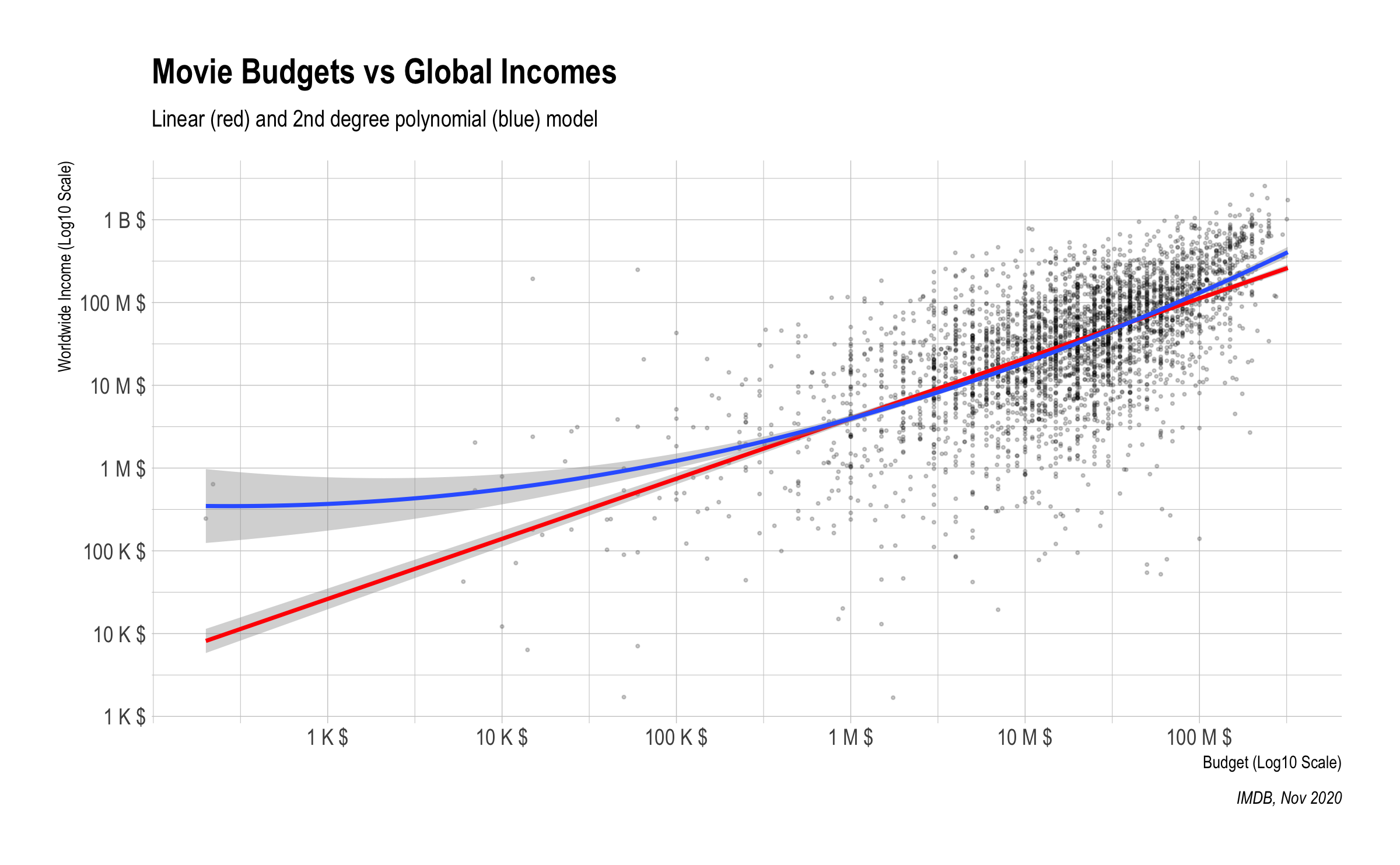
During the exploratory data analysis, the clear correlation between budget and income was observed. For modelling of that relation 4 different models were used and compared to their adj.r.squared value. As expected, the linear model was best when both budget and income was at logarithmic scale.
#> # A tibble: 4 x 3
#>   model                         r_squared adj_r_squraed
#>   <chr>                             <dbl>         <dbl>
#> 1 Linear Model                      0.405         0.405
#> 2 Polynomial Model (2nd degree)     0.416         0.415
#> 3 Polynomial Model (3rd degree)     0.416         0.415
#> 4 Linear Model (Log)                0.389         0.389
#>
#> Call:
#> lm(formula = profit ~ poly(budget, degree = 2), data = drop_na(movies_df,
#> budget))
#>
#> Residuals:
#> Min 1Q Median 3Q Max
#> -6.96e+08 -4.11e+07 -2.19e+07 1.38e+07 1.89e+09
#>
#> Coefficients:
#> Estimate Std. Error t value Pr(>|t|)
#> (Intercept) 9.74e+07 2.12e+06 45.96 <2e-16 ***
#> poly(budget, degree = 2)1 6.53e+09 1.29e+08 50.67 <2e-16 ***
#> poly(budget, degree = 2)2 1.05e+09 1.29e+08 8.11 7e-16 ***
#> ---
#> Signif. codes: 0 '***' 0.001 '**' 0.01 '*' 0.05 '.' 0.1 ' ' 1
#>
#> Residual standard error: 1.29e+08 on 3701 degrees of freedom
#> Multiple R-squared: 0.416, Adjusted R-squared: 0.415
#> F-statistic: 1.32e+03 on 2 and 3701 DF, p-value: <2e-16According to predicted best model (Polynomial Model (2nd degree)), each unit increase of the budget significantly (p < 2e-16) increase the profit variable. So, budgets positively correlate with profits. While, the polynomial model is slightly better according the adjusted r squared value (explains %1 more of the outcome variability compared to linear model), the linear model is preferred for the rest of the analysis as it is more easier to interpret and comment. The graph below also shows that both model has similar trend in the majority of the data.

According to our model, it can be observed that the budget accounts for more than 40% of global incomes, with p-values close to zero, meaning the relationship is statistically significant at any level.
It appears to be more difficult to predict financial success for lower budget films (i.e., less than $1 million) which is certainly good news for the industry, leaving room for new studios to emerge on the market if things are done with talent. To explain this, let’s imagine that each film produced would be a company, there would be a spectrum ranging from startups (i.e. films with less than 10 million budget) to huge multinationals (i.e. films With a budget exceeding 100 million), it is therefore easier to understand from this angle that low-budget films manage in some cases to produce exceptional financial results thanks to, among other things, ideas, better execution or the possibility of risking more (since they have less to lose).
Afterwards, however, a leap seems to appear for those wishing to make a place for themselves among big players of the market with budgets above $100 million, where money seems to count more (as suggests the 2nd degree polynomial model), and which seems in the end to be typical of any other industry where more means generally means more income.
Moreover, Those big players have a better customer knowledge; they also know better which movie will be a good one by analysing all the insights they gathered through the years. They will also take more time to analyze whether their idea is really a good one; reputation plays a big role for those companies, a bad movie can have huge negative consequences.
In other words, it can be observed in the 2nd degree polynomial model (blue) that once the 100 million budget mark is passed, the budget-profit correlation tends to be even stronger. Again, let’s compare any high-budget film (i.e., with 90 - 100 million budget or more) to a multinational company with the experience and industry expertise to go with it, which knows the expectations of the audience and will more rarely experience failures when launching new products (in our case films). We can therefore draw the intermediate conclusion that although made of rhinestones and glitter, the film industry is subject to the same economic rules as any other industry where competition is tough.
Does this prediction change regarding the movie genre?
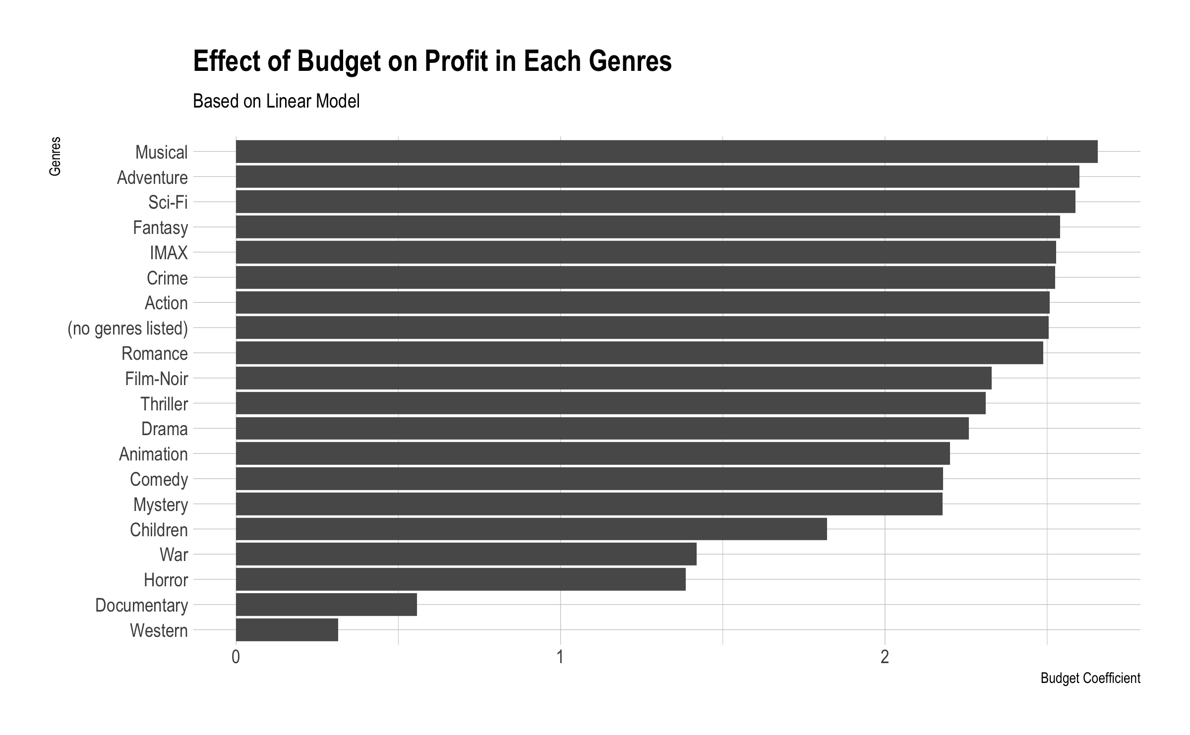
To understand the relation between budget and profit in different genres, same linear modelling was applied in each genres seperately. The table below shows the coefficients of the budget in different genres. Except documentary and western genres, most ot the categories have similar coefficients. As a result, the prediction changes regarding the movie genres.

However, as the table shows, the p-values for the western (0.16445) and documentary (0.31132) genres are not significant at any common level of alpha, thus not allowing us for these two genres to reject the null hypothesis that a change in the budget would have no impact on profits. As far as the other genres are concerned, the p-values all allow to reject the null hypothesis that there would be no correlation between budget and income by taking these genres into account, at any alpha level.
We can therefore classify the genres into three clusters:
Group 1: Musical, Adventure, Science-Fiction, Fantasy, IMAX, Crime, Action & Romance.
Group 2: Black Film, Thriller, Drama, Animation, Comedy & Mystery.
Group 3: Children, War & Horror.
Cluster 1 includes the genres where the budget correlates the most with revenues while on the other side Cluster 3 includes the genres where the budget effect has the least impact on profits. This result seems relevant from the point of view of either an investor or a film production studio seeking to maximize its profits; It seems wiser for investors to fund movies having a genre included in Cluster 1.
Does this prediction change based on the gender type of the main characters?
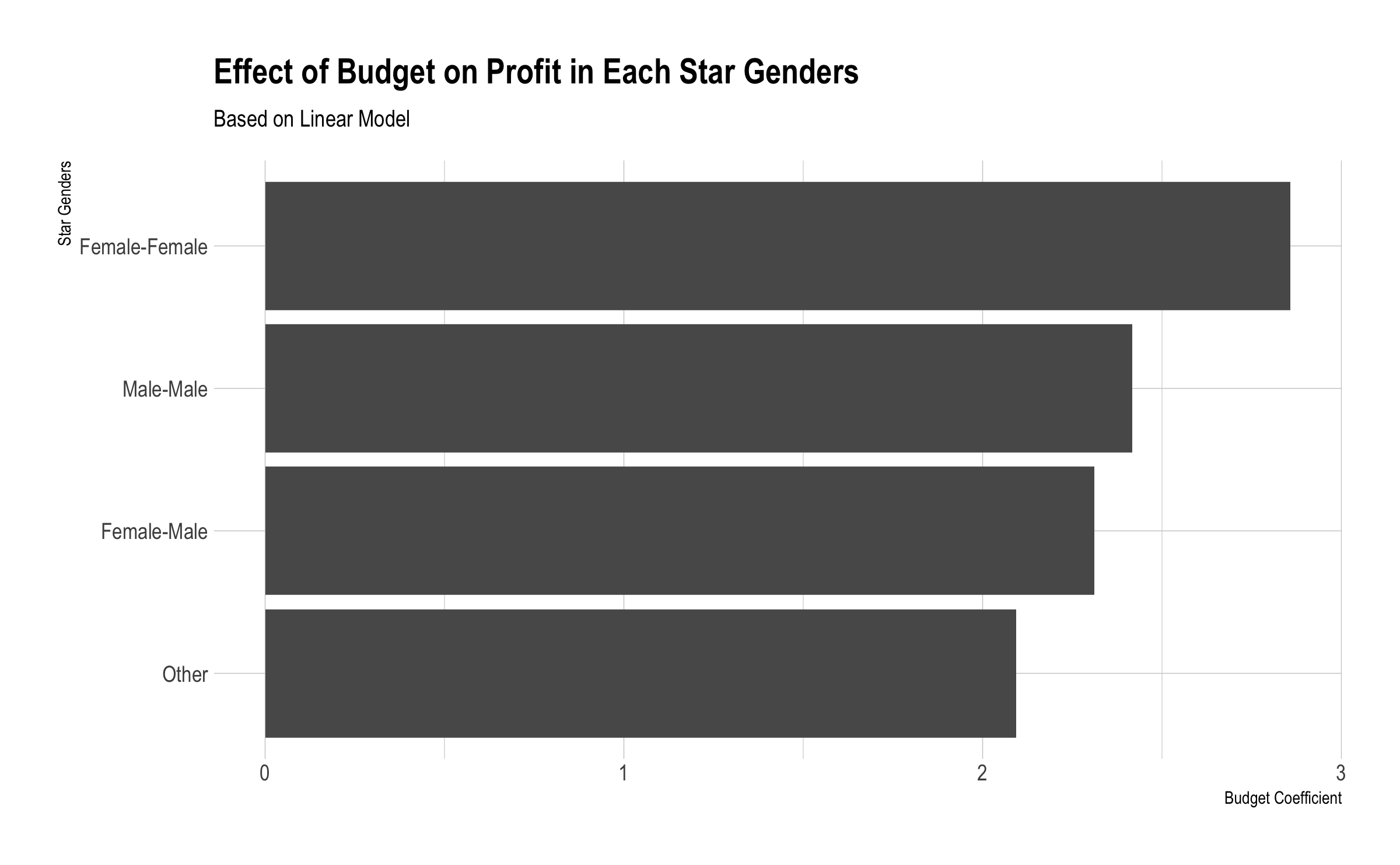
Similary, to identify the budget - profit relation for the star genders, linear modelling was applied in each star gender categories (male-female, female-female, female-male) seperately. The table below shows the coefficients of the budget in different star gender categories. The table below shows the budget coefficients on profit for each category.

Here, our results go against the “common belief” that films with men as main characters would be more successful (disclaimer: does not represent our personal point of view) and therefore the effect of the budget on the film’s profit would be greater, always by taking the genre of the main characters in consideration. Although our results do not allow us to draw too hasty conclusions, that our preliminary results would certainly deserve a whole dedicated project, it is still relevant in our context to take this into account. In short, an important signal to draw from this would certainly be that the public expects a certain diversity on the screen with regard to the genre of the main characters.
Can we see differences in the effect regarding the movie production studio?
As majority of the studios have 2 or less movies in the given dataset, the linear model couldn’t be applied on those. In the table below, the budget coeffients and other statistics were shown for each studio. The test showed that, in the scope of most of the studios, the budget coefficient and relation significance vary a lot.
Therefore, although the initial belief was to be able to predict a correlation between budget and profit depending on the studio that produced the film, our results are disappointing on this side, with p-values generally too large, therefore statistically insignificant to allow us to reject the null hypothesis, at least with our sample data. Our model shows that there is not any significant difference of the correlation when compared to different production studios. This result is also really important; it means that studios that have less popularity still can make a successful movie if they have a good budget. It also explains why there are a lot of competitors still staying in the market even if there are big players; if the best production studios could make more profits when investing a lot of money, then the other competitors would not survive.
Does this prediction change based on the year?
As we did on the previous comparisons, to determine the changes on budget - profit relation over years, linear modelling was applied in each star years seperately. The table below shows the coefficients of the budget in different years. As the numbers of movies before 1975 was too low, those are omitted from analysis.
#> Warning: All elements of `...` must be named.
#> Did you want `data = c(movieId, title, genres, budget, profit, studio, star_female,
#>     star_male, star_unknown)`?
The graph shows that after the begining of 2000’s, the effect of bugget on the income started to increase slightly.
Thus, we can first observe a decreasing trend in the 1990s through the early 2000s in the effect of the budget on revenues before a reversal of this trend that continues to the present day. First of all, in the 1990s technological changes made film production more accessible and cheaper compared to before, which is one of the reasons of the decreasing trend observed in those years. Then the trend was reversed at the beginning of the 2000s years, with the success of blockbusters and the madness that gripped the film industry to always want to do more, higher and bigger.
This can be demonstrated by the fact that the 42 most expensive productions in history have all been produced in the years 2000 - 2020. Titanic (1997) being ranked 43rd most expensive production with its $200 million budget and first most expensive film for films produced before the 2000s.
Moreover, it was also technological advances that had brought the trend down before reaching a plateau, which may partly explain the fact that this trend has started up again, since the technological advances and means put into production and post-production have radically transformed the cinematographic landscape.