2 K-means clustering

2.1 Introduction

K-means clustering is a popular unsupervised learning method based on a simple and intuitive approach that clusters similar observations into groups.

We start by choosing the number of clusters $K$ and the objective is to assign every observation to one, and just one, of the clusters. The clusters are chosen so that the within-cluster variation is minimised, i.e., the data points in each cluster should be close together.

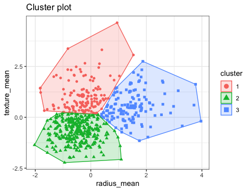
The figure below shows an example of 3 clusters based on two variables.

The way the clusters are defined is based on an iterative process. Once we chose the number of clusters,

we start by assigning each data point to one of the clusters, randomly.
We then compute the centroid of each cluster.
Next, we compute the distance (usually the Euclidean distance) of each data point to the centroids.
The data points are re-assigned to the corresponding cluster of the closest centroid.
The centroids are recomputed
We repeat the process until convergence

One important question that immediately arises is how many clusters should we consider ? Unfortunately, there is not a definitive answer. In the practice session we will show some graphical methods that can be used as an indication of the number of clusters suggested by the data, but as you will see, different methods can suggest different number of clusters.

2.2 Readings

Read the following chapters of An introduction to statistical learning:

10.3.1 K-Means Clustering Analysis

2.3 Practice session

TASK 1 - Identify k clusters

Using the bdiag.csv, let’s use 2 of the variables that characterise the cell nuclei - radius_mean and texture_mean - to identify 3 data clusters

We will use the function kmeans() with the option centers=3 indicating that we want 3 clusters.

#read the dataset
bdiag.data <- read.csv("https://www.dropbox.com/s/vp44yozebx5xgok/bdiag.csv?dl=1", 
           stringsAsFactors = TRUE)

#select a subset of the variables
bdiag.2vars <- bdiag.data[,c("radius_mean", "texture_mean")]

#let's compute the 3 clusters
km <- kmeans(bdiag.2vars, centers = 3)

km

## K-means clustering with 3 clusters of sizes 305, 130, 134
## 
## Cluster means:
##   radius_mean texture_mean
## 1    12.36637     16.31328
## 2    19.33692     21.52369
## 3    13.08123     23.89687
## 
## Clustering vector:
##   [1] 1 2 2 3 2 1 2 3 3 3 3 1 2 3 3 3 3 2 2 1 1 1 1 2 2 1 3 2 3 1 2 1 2 2 1 2 3
##  [38] 1 3 3 3 3 2 3 3 2 1 1 1 3 3 1 1 2 3 1 2 3 1 1 1 3 3 1 3 3 3 1 1 1 2 1 2 1
##  [75] 1 2 1 2 2 1 3 1 2 2 1 2 3 2 3 1 3 3 1 1 1 2 1 1 1 1 3 1 3 1 1 1 1 1 2 3 1
## [112] 3 1 1 1 3 1 1 3 2 1 2 2 1 1 1 3 2 1 2 1 2 2 1 2 3 1 1 1 1 1 1 1 1 1 1 1 1
## [149] 1 1 3 3 1 1 1 1 2 2 1 1 1 2 2 3 2 1 1 2 2 1 1 1 1 1 1 1 1 2 3 1 2 2 2 1 3
## [186] 1 2 1 1 1 3 3 1 3 3 1 3 2 2 3 1 2 2 3 1 1 1 2 3 1 2 1 2 2 3 1 1 1 2 3 1 1
## [223] 1 2 1 1 1 1 3 3 2 3 3 2 1 3 2 2 3 3 1 1 1 3 2 1 1 1 3 1 2 1 2 2 2 1 2 1 3
## [260] 3 2 2 2 2 2 2 1 3 1 3 1 1 2 1 2 1 1 2 1 1 2 1 2 2 1 1 3 1 1 1 1 1 1 1 1 1
## [297] 1 1 1 3 2 1 2 1 1 3 1 1 1 1 1 1 1 1 1 1 1 2 1 1 1 2 1 2 1 1 1 1 2 2 1 1 1
## [334] 1 1 2 1 2 1 2 1 1 1 2 1 1 1 1 1 1 1 2 2 3 1 1 1 1 1 1 1 3 1 2 1 2 2 1 2 2
## [371] 3 1 2 2 1 1 1 3 1 1 1 1 3 1 1 3 1 1 1 2 1 1 2 2 1 1 1 1 1 1 2 1 1 1 1 1 1
## [408] 3 2 1 1 1 3 3 3 3 3 3 1 3 1 1 1 1 1 3 1 3 1 1 3 1 2 2 1 1 1 1 1 1 1 2 1 1
## [445] 2 3 3 1 1 2 3 2 3 1 1 3 3 3 3 3 3 2 3 1 1 3 3 1 2 1 1 3 1 3 1 1 3 1 1 2 1
## [482] 1 1 1 1 1 1 2 1 2 3 1 2 1 3 3 1 1 2 2 1 3 1 2 1 1 1 1 1 3 1 1 3 1 1 1 2 2
## [519] 1 1 1 2 1 1 1 1 1 1 1 1 1 1 1 2 1 2 3 3 3 3 1 3 3 3 3 3 1 1 1 3 3 3 3 3 3
## [556] 3 1 3 3 3 3 3 3 2 2 2 3 2 3
## 
## Within cluster sum of squares by cluster:
## [1] 2653.828 2032.052 2059.736
##  (between_SS / total_SS =  61.6 %)
## 
## Available components:
## 
## [1] "cluster"      "centers"      "totss"        "withinss"     "tot.withinss"
## [6] "betweenss"    "size"         "iter"         "ifault"

The component km$cluster has the final clusters assignment. We will use the package factoextra that has some plot functions (based on ggplot) that are useful.

The fviz_cluster() plots the results of the clusters in a scatter plot formed by the two variables. If the clustering is based on more than 2 variables, this function will run a principal components analysis and plot the first 2 principal components.

library(factoextra)
fviz_cluster(km, data = bdiag.2vars, label=NA)+theme_bw()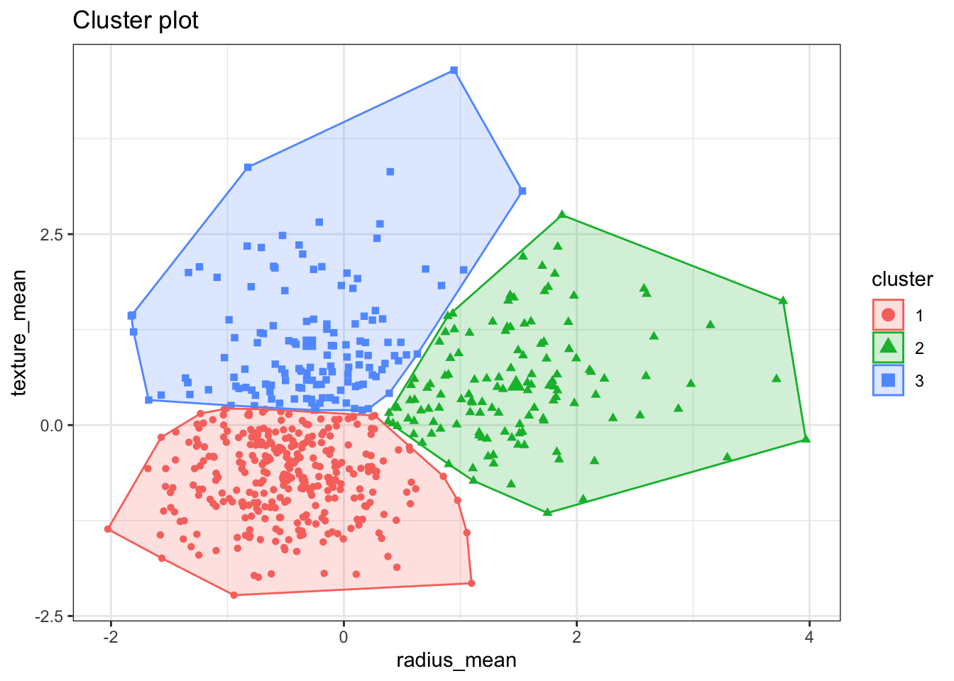

TRY IT YOURSELF:

Get 2 clusters with k-mean clustering based on the variables age, weight, height, adipos, free, neck, chest, abdom, hip, thigh, knee, ankle, biceps, forearm and wrist .

See the solution code

#select a subset of the variables
bdiag.10vars <- bdiag.data[,c("radius_mean", "texture_mean",  
                     "perimeter_mean", "area_mean", 
                     "smoothness_mean", "compactness_mean", 
                     "concavity_mean", "concave.points_mean", 
                     "symmetry_mean", "fractal_dimension_mean")]
k2 <- kmeans(bdiag.10vars, centers = 2)
fviz_cluster(k2, data = bdiag.10vars, label=NA)+theme_bw()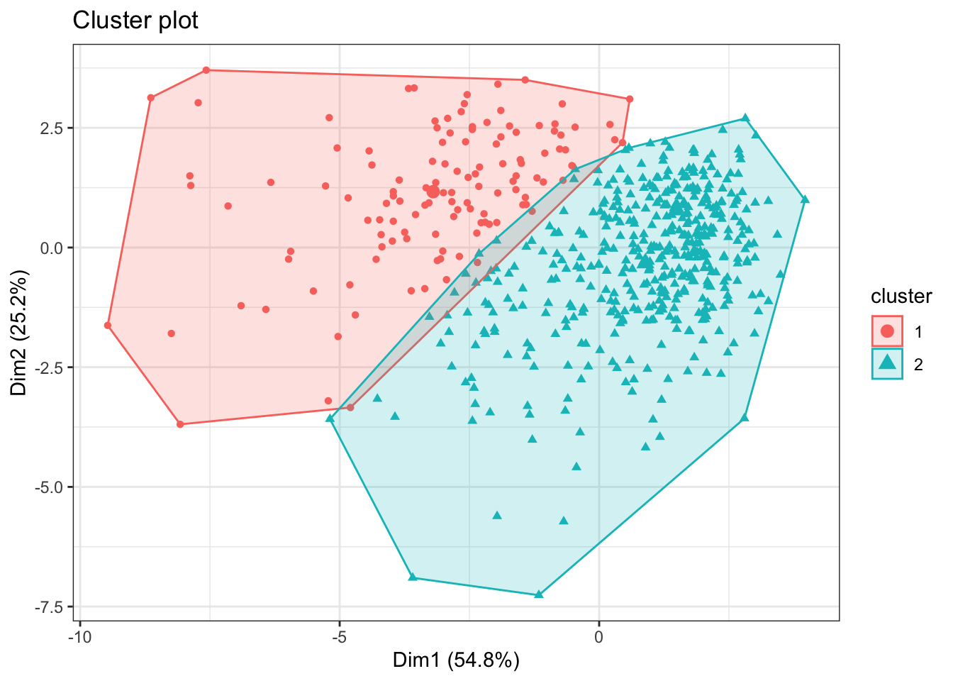

TASK 2 - Choosing the number of clusters

Lets consider the same example as in Task 1 with two variables.How many clusters should we consider?

There are some ad-hoc visual methods that may help you guide selecting the number of clusters.

The first method is called the Elbow method and consists in

computing the k-means clustering for different values of $k$, e.g, by varying $k$ from 1 to 10 clusters
then, for each k, calculate the total within-cluster sum of square ($wss$)
and finally, plot the curve of $wss$ according to the number of clusters $k$.

In the plot, the location of a bend (knee) suggests the appropriate number of clusters. The function fviz_nbclust() implements this method

fviz_nbclust(bdiag.2vars, kmeans, method = "wss",  k.max = 10)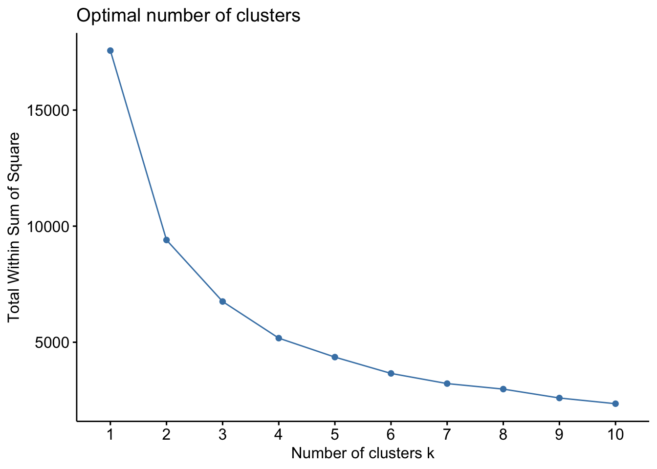

The plot above suggest 2 or 3 clusters.

Another method is the Average Silhouette Method. In this method we look at the quality of the clustering by measuring how well each data point lies within its cluster. If the average silhouette width is high, this suggests a good clustering. We can then compute the average silhouette width for different values of $k$ and select the number of clusters with higher average silhouette width.

The same function as above also implements this method.

fviz_nbclust(bdiag.2vars, kmeans, method = "silhouette",  k.max = 10)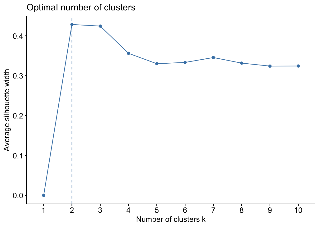

This method suggests 2 clusters.

The final method is the Gap Statistic Method. This method compares the total intracluster variation for different number of cluster $k$ with their expected values under a data with no clustering (these data generated using Monte Carlo simulations). The higher the gap between the observed and expected, the better the clustering. More details about this method is available in R. Tibshirani, G. Walther, and T. Hastie (Standford University, 2001)

fviz_nbclust(bdiag.2vars, kmeans, method = "gap",  nboot=200, k.max = 10)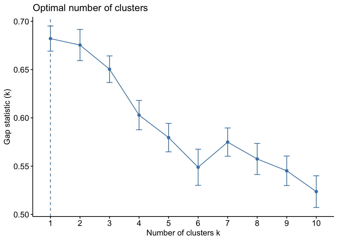

In this case, the method suggests 1 single cluster.

Depending on the method used, we could have selected between 1 to 3 clusters.

2.4 Exercises

Solve the following exercises:

The dataset fat is available in the library(faraway).
The data set contains several physical measurements.

Using the variables age, weight, height, adipos, free, neck, chest, abdom, hip, thigh, knee, ankle, biceps, forearm and wrist

Plot 3 clusters produce by k-mean in the scatter plot formed by the two principal components of the data?
Use different methods to investigate how many clusters are suggested by the data.