3 Text Analytics with R: Topic Modelling
This tutorial introduces text analyses in R using a variety of R packages and tidy tools.
3.1 Initial R Setup
3.1.1 Load the R Packages
Load and import the necessary R packages:
library(readr)
# a collection of package for data wrangling.
library(tidyverse)
# package for text processing
library(tidytext)
# collection of packages for modeling and L
library(tidymodels)
library(scales)
# R package for managing and analyzing textual data
library(quanteda)
# An R package with word stemming algorithm
# collapsing words to a common root to aid comparison of vocabular.
library(SnowballC)
# library for topic models (LDA)
library(topicmodels)
# text recipe
library(textrecipes)
# dealing with imbalance data using `step_downsample or upsample`.
library(themis)
# https://github.com/tidymodels/discrim
library(discrim)
# framework for constructing variable importance plots from ML models
library(vip)
3.1.2 Load the Twitter Data for Topic Modelling
We start from data loading and text pre-processing.
urlfile_tm <-"https://raw.githubusercontent.com/tianyuan09/ai4ph2022/main/sampleTwitterDataForTopicModelling.csv"
tweetsTMDF <-read.csv(url(urlfile_tm), encoding = "UTF-8")

### UDF to remove the URLs from the tweets
removeURLs <- function(tweet) {
  return(gsub("http\\S+", "", tweet))
}
### UDF to remove RT from the tweets
removeUsernamesWithRT <- function(tweet) {
  return(gsub("^RT @[a-z,A-Z]*[0-9]*[a-z,A-Z]*[0-9]*: ","", tweet))
}
### UDF to remove the usernames or callouts from the tweets
removeUsernames <- function(tweet) {
  return(gsub("@[a-z,A-Z]*[0-9]*[a-z,A-Z]*[0-9]*", "", tweet))
}
### remove the hashtag # from the tweets
removeHashtagSignOnly <- function(tweet) {
  return(gsub("#", "", tweet))
}

# pre-processing using regex
tweetsTMDF$processed_tweet <- apply(tweetsTMDF['tweet'], 2,
                                    removeURLs)
tweetsTMDF$processed_tweet <- apply(tweetsTMDF['processed_tweet'],2,
                                    removeUsernamesWithRT)
tweetsTMDF$processed_tweet <- apply(tweetsTMDF['processed_tweet'],2,
                                    removeUsernames)
tweetsTMDF$processed_tweet <- apply(tweetsTMDF['processed_tweet'],2,
                                    removeHashtagSignOnly)

# pre-processing tokenization, stopword, stemming
text_tmdf <- tweetsTMDF %>% select(X,processed_tweet) %>%
    unnest_tokens(word, processed_tweet)%>%
  anti_join(stop_words[stop_words$lexicon == "snowball",], by = "word")%>%
  mutate(stem = wordStem(word))


#  we can tokenize text into consecutive sequences of words, called n-grams
text_bigrams<-tweetsTMDF %>% select(X,processed_tweet) %>%
  unnest_tokens(bigram, processed_tweet, token="ngrams", n=2)%>%
  filter(bigram != "covid 19")
3.2 Topic Modelling
Topic modelling is an unsupervised machine learning approach that can scan a collection of documents, find word and phrase patterns within them, and automatically cluster word groupings and related expressions into topics.
What is topic modelling?
Topic modeling, including probabilistic latent semantic indexing and latent Dirichlet allocation, is a form of dimension reduction that uses a probabilistic model to find the co-occurrence patterns of terms that correspond to semantic topics in a collection of documents (Crain et al. 2012).
Topic models require a lot of subjective interpretation when it comes:
- the choice of K topics. There is no clear criteria for determining the number of topics K. When it comes to interpretability or coherence of topics, top words might help. You should always inspect topics manually, think carefully about theoretical concepts that you can measure with topics.
- the identification and exclusion of background topics
- the interpretation and labeling of topics identified as relevant
- the “assignment” of topics to documents
3.2.1 Latent Dirichlet allocation (LDA)
Latent Dirichlet allocation (LDA) is the one of the most common algorithms for topic modelling, and it is guided by two principles:
- Each document has a mixture of topics.
- Each topic is a mixture of words.
LDA estimate both of these at the same time and find the mixture of words that associated with each topic.
Create a document-term-matrix using the cast_dfm(). More information about tidy text format can be found at here (Silge and Robinson 2017)
# create a document term (or feature) matrix
word_counts_dtm = text_tmdf %>% count(X, word) %>%
  cast_dfm(X, word, n)
word_counts_dtm
## Document-feature matrix of: 12,808 documents, 16,728 features (99.94% sparse) and 0 docvars.
##     features
## docs agree also don’t everyone isolating masks one way wearing fort
##   18     1    1     1        1         1     1   1   2       1    0
##   30     0    0     0        0         0     0   0   0       0    1
##   31     0    0     0        0         0     0   0   0       0    0
##   38     0    0     0        0         0     0   0   0       0    0
##   47     0    0     0        0         0     0   0   0       0    0
##   57     0    0     0        0         0     1   0   0       1    0
## [ reached max_ndoc ... 12,802 more documents, reached max_nfeat ... 16,718 more features ]

# check the top features in our dataset
topfeatures(word_counts_dtm, n = 20, scheme = "docfreq")
##        covid           19     pandemic        cases          new      covid19
##         4784         3213         1328          892          873          826
## saskatchewan         sask  coronavirus      vaccine       people         mask
##          822          799          780          763          708          608
##         will          get          can        masks          one   vaccinated
##          544          494          480          470          460          449
##          now       health
##          440          434

# bigram matrix
bigrams_counts_dtm = text_bigrams %>% count(X,bigram)%>%
  cast_dfm(X, bigram, n)
bigrams_counts_dtm
## Document-feature matrix of: 12,776 documents, 96,879 features (99.99% sparse) and 0 docvars.
##     features
## docs a way agree that also be be a don’t agree everyone wearing i don’t is only
##   18     1          1       1    1           1                1       1       1
##   30     0          0       0    0           0                0       0       0
##   31     0          0       0    0           0                0       0       0
##   38     0          0       0    0           0                0       0       0
##   47     0          0       0    0           0                0       0       0
##   57     0          0       0    0           0                0       0       0
##     features
## docs masks would one way
##   18           1       1
##   30           0       0
##   31           0       0
##   38           0       0
##   47           0       0
##   57           0       0
## [ reached max_ndoc ... 12,770 more documents, reached max_nfeat ... 96,869 more features ]

topfeatures(bigrams_counts_dtm, n = 20, scheme = "docfreq")
##          of covid            in the            of the         the covid
##               549               505               466               327
##      the pandemic            to the         new cases   in saskatchewan
##               314               301               294               274
## social distancing          19 cases             19 in            a mask
##               258               252               239               234
##            due to          cases of           for the             to be
##               230               227               222               220
##            on the          to covid           in sask           this is
##               210               210               205               203
We can use the LDA() function from the topicmodels to create a two-topic model. In reality, you may need to try different values of k.
tweet_lda2 <- LDA(word_counts_dtm, k = 2, control = list(seed = 1234))
tweet_lda2
## A LDA_VEM topic model with 2 topics.
#The terms that are particularly strongly linked to each of the topics
as.data.frame(terms(tweet_lda2, 15))
##         Topic 1     Topic 2
## 1         covid          19
## 2            19    pandemic
## 3         cases       covid
## 4          mask        sask
## 5          will     vaccine
## 6       covid19         new
## 7  saskatchewan coronavirus
## 8           new         get
## 9        people        like
## 10          one       cases
## 11       health        news
## 12           sk         can
## 13  coronavirus       masks
## 14         says      people
## 15          day        just
We can use the LDA() function from the topicmodels to create a four-topic model using the bi-gram.
tweet_lda4 <-LDA(bigrams_counts_dtm, k = 4, control = list(seed = 1234))
tweet_lda4
## A LDA_VEM topic model with 4 topics.
#The terms that are particularly strongly linked to each of the topics
as.data.frame(terms(tweet_lda4, 15))
##            Topic 1           Topic 2         Topic 3      Topic 4
## 1        new cases social distancing           to be       of the
## 2         of covid         for covid      details at     of covid
## 3           in the            in the          in the    the covid
## 4         cases of            a mask      a pandemic the pandemic
## 5            19 in      the pandemic       gx94 news       in the
## 6  in saskatchewan            to the        of covid   during the
## 7           of the         the covid in saskatchewan       on the
## 8          in sask              i am          due to      this is
## 9        new covid            is the          to the     with the
## 10        19 cases             19 in          a mask     to covid
## 11          to the           in sask          have a         is a
## 12       the covid          on covid          of the  the vaccine
## 13         for the   the coronavirus        to covid     19 cases
## 14        total to          of covid            in a       to the
## 15        cases in            of the         have to      for the
3.2.1.1 Word-topic probabilities
The tidytext package has method for extracting the per-topic-per-word probabilities, the beta, from the two-topic model.
lda_topics <-tidy(tweet_lda2,matrix="beta")
lda_topics
## # A tibble: 33,456 x 3
##    topic term           beta
##    <int> <chr>         <dbl>
##  1     1 agree     0.000325
##  2     2 agree     0.000263
##  3     1 also      0.000972
##  4     2 also      0.00179
##  5     1 don’t     0.00136
##  6     2 don’t     0.00153
##  7     1 everyone  0.00114
##  8     2 everyone  0.00104
##  9     1 isolating 0.0000790
## 10     2 isolating 0.000117
## # ... with 33,446 more rows

lda_topics4 <-tidy(tweet_lda4,matrix="beta")
lda_topics4
## # A tibble: 387,516 x 3
##    topic term            beta
##    <int> <chr>          <dbl>
##  1     1 a way      2.07e-  5
##  2     2 a way      5.74e-  5
##  3     3 a way      8.99e-  5
##  4     4 a way      2.19e-  4
##  5     1 agree that 7.87e-197
##  6     2 agree that 4.57e-  5
##  7     3 agree that 1.93e- 10
##  8     4 agree that 6.92e-  5
##  9     1 also be    2.12e-  5
## 10     2 also be    1.59e-201
## # ... with 387,506 more rows
Find the 15 terms that are most common within each topic.dplyr’s slice_max()
ap_top_terms <- lda_topics %>%
  group_by(topic) %>%
  slice_max(beta, n = 15) %>%
  ungroup() %>%
  arrange(topic, -beta)

ap_top_terms %>%
  mutate(term = reorder_within(term, beta, topic)) %>%
  ggplot(aes(beta, term, fill = factor(topic))) +
  geom_col(show.legend = FALSE) +
  facet_wrap(~ topic, scales = "free") +
  scale_y_reordered()+
  labs(title = "The terms that are most common within each topic")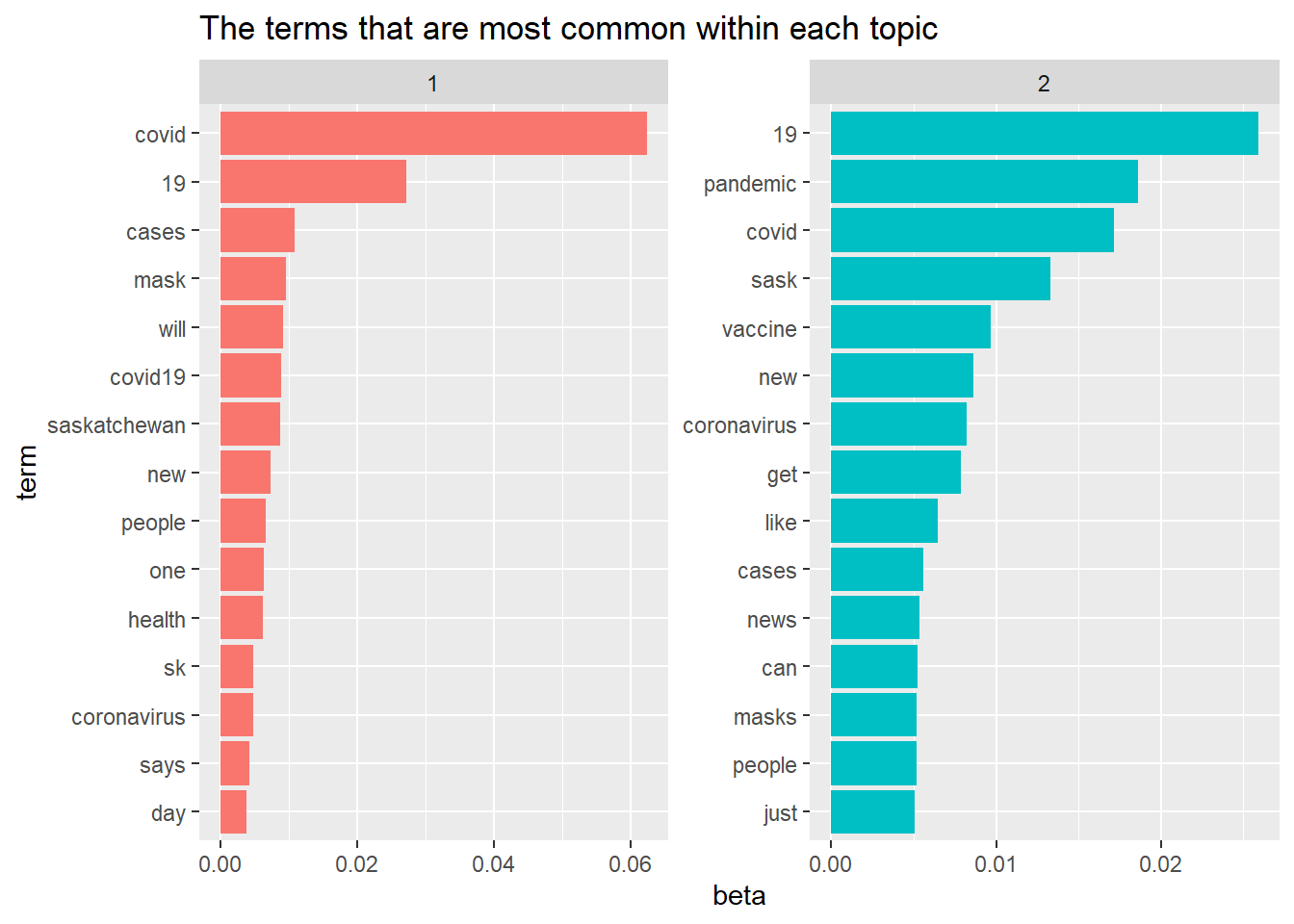
Find the 15 terms that are most common within each topic.dplyr’s slice_max()
ap_top_terms4 <- lda_topics4 %>%
  group_by(topic) %>%
  slice_max(beta, n = 15) %>%
  ungroup() %>%
  arrange(topic, -beta)

ap_top_terms4 %>%
  mutate(term = reorder_within(term, beta, topic)) %>%
  ggplot(aes(beta, term, fill = factor(topic))) +
  geom_col(show.legend = FALSE) +
  facet_wrap(~ topic, scales = "free") +
  scale_y_reordered()+
  labs(title = "The terms that are most common within each topic")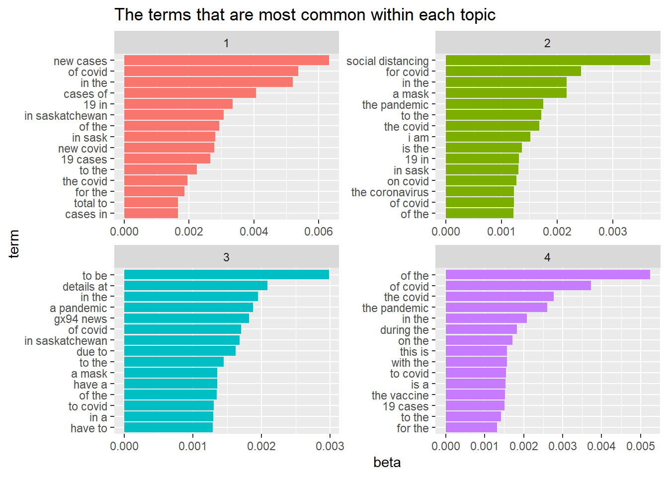
Find the terms that generate the greatest difference in beta between two topics.
beta_wide <- lda_topics %>%
  mutate(topic = paste0("topic", topic)) %>%
  pivot_wider(names_from = topic, values_from = beta) %>%
  filter(topic1 > .001 | topic2 > .001) %>%
  mutate(log_ratio = log2(topic2 / topic1))

beta_wide %>% arrange(desc(abs(log_ratio)))%>% head(20) %>%
    arrange(desc(log_ratio)) %>%
    ggplot(aes(log_ratio, term)) +
    geom_col(show.legend = FALSE)+
    labs(title = "Terms with the great difference in beta between two topics")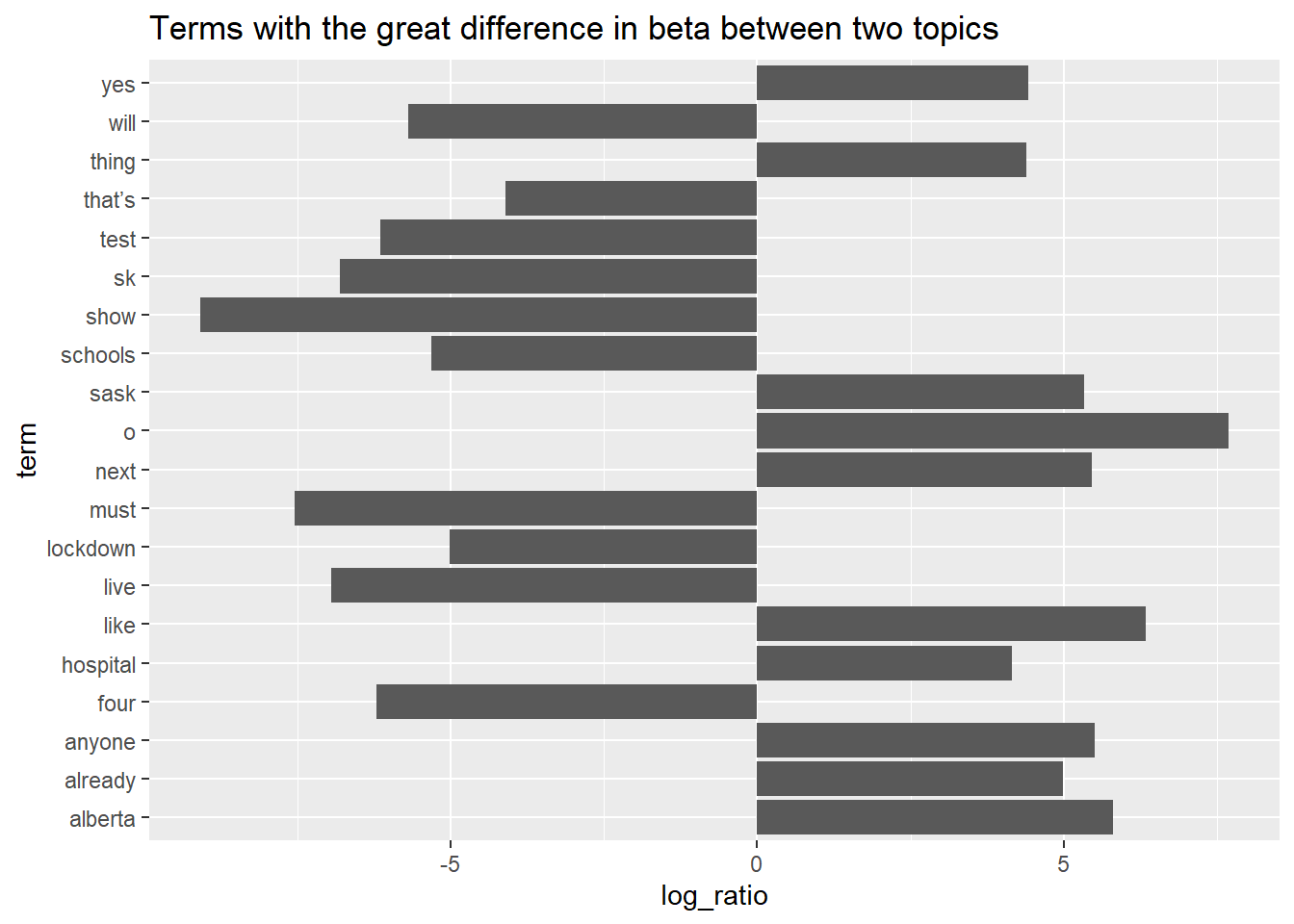
3.2.1.2 Document-topic probabilities
LDA models each document as a mix of topics and words. With matrix = "gamma", we can investigate per-document-per-topic probabilities.
lda_documents <- tidy(tweet_lda2, matrix = "gamma")
lda_documents
## # A tibble: 25,616 x 3
##    document topic gamma
##    <chr>    <int> <dbl>
##  1 18           1 0.512
##  2 30           1 0.512
##  3 31           1 0.510
##  4 38           1 0.500
##  5 47           1 0.514
##  6 57           1 0.507
##  7 95           1 0.520
##  8 100          1 0.501
##  9 163          1 0.475
## 10 175          1 0.490
## # ... with 25,606 more rows
Each of these values represents an estimated percentage of the document’s words that are from each topic. Many of these tweets were drawn from more than 1 topic.