Statistical Modeling II: SDS383D
2023-03-22
Chapter 1 Introduction to Probabilistic Modeling
In this collection of notes, we briefly outline the main thrust of this course by discussing (at a high level of generality) the topic of probabilistic modeling. Throughout this course we will focus on the application of probabilistic modeling with an eye towards solving problems involving complex datasets. The following problems will recur throughout:
How do we design an appropriate probabilistic model that answers the questions we are interested in?
Computationally, how do we extract answers from a probabilistic model?
How do we properly account for uncertainty in our conclusions?
How do we check that our model is “good enough” as a representation of reality for our purposes, and ensure that the conclusions we draw are robust?
1.1 Very Simple Probabilistic Models
At this stage in your education, you are undoubtedly familiar with the concept of probabilistic modeling. All this means is that:
We have a collection \(\mathcal D\) of data that we have measured.
We posit that \(\mathcal D\) has arisen by randomly sampling it according to some data generating process \(G\), i.e., \(\mathcal D\sim G\).
That’s it! The most generic probabilistic model stops after Step 2. Such a model is not very useful, however; for example, if \(\mathcal D= (X_1, \ldots, X_N)\) and all we know is that \(G\) is an arbitrary probability distribution on \(\mathbb R^N\), then it will be more-or-less impossible to draw any conclusions about \(G\) from the data. Generally we assume more.
Example 1.1 (IID Sampling) Suppose that \(\mathcal D= (X_1, \ldots, X_N)\) and suppose further that \(X_i \stackrel{\text{iid}}{\sim}F\) so that \(G = F^N\). Then a reasonable estimate of \(F\) is the empirical distribution \[ \mathbb F_N = \frac{1}{N} \sum_{i = 1}^N \delta_{X_i}, \] where \(\delta_{X_i}\) denotes the point mass distribution at \(X_i\). We make no assumptions about \(F\) itself; it can be (say) a normal distribution, an exponential distribution, a Cauchy distribution, or any other distribution.
Part of the point of brining up this example is to point that, while weak, the assumption that a collection of data is iid is an assumption that should be scrutinized. Data might fail to be iid if (for example) the \(X_i\)’s correspond to a time series.
Already in Example 1.1 interesting problem start occurring. For example, suppose we know that \(F\) has a density \(f(x)\) that we are interested in estimating. How do we go about estimating \(f(x)\) within the context of the iid model?
Example 1.2 (Density Estimation) The galaxy dataset available in the MASS package contains “a numeric vector
of velocities in km/sec of 82 galaxies from 6 well-separated conic sections of
an unfilled survey of the Corona Borealis region. Multimodality in such surveys
is evidence for voids and superclusters in the far universe.”
Our primary goal is to determine whether the density \(f(x)\) of the velocities is multimodal. We’ll assume that the sample of galaxies is taken iid from some distribution \(Y_i \stackrel{\text{iid}}{\sim}F\) with density \(f(y)\). We then form the density estimate \[\begin{align*} \widehat f(y) = \frac{1}{N} \sum_i \phi(y; Y_i, h) \end{align*}\] where \(\phi(y; \mu, \sigma)\) denotes the density of a \(\operatorname{Normal}(\mu, \sigma^2)\) distribution. This estimator is biased and, in fact, there are no unbiased estimators of \(f(y)\) if we make no further assumptions on \(F\). A plot of the density estimate is given in Figure 1.1.
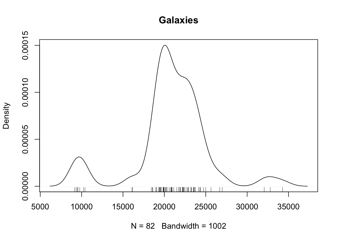
Figure 1.1: Density estimate for the galaxy dataset.
The estimator \(\widehat f(y)\) described in Example 1.2 is called a kernel density estimator (KDE). KDEs are biased and, in general, there is no way around this. The introduction of bias is a concession we make in order to make progress on our problem. All interesting problems require some form of concession; a common concession is to assume that the data arise from a parametric family.
Example 1.3 (Linear Regression) Suppose that \(\mathcal D= \{(x_1, Y_1), \ldots, (x_N, Y_N)\}\) with the \(x_i\)’s being fixed vectors in \(\mathbb R^P\), with \(G\) satisfying the restrictions \[\begin{align*} Y_i = r(x_i) + \epsilon_i, \qquad \operatorname{Var}(\epsilon_i) = \sigma^2 < \infty. \end{align*}\] Without making further assumptions, this sort of problem arises frequently in various machine learning problems, with the goal of estimating the mean function \(r(x)\) to provide predictions on new data. As statisticians, we often make the further assumption that \[\begin{align} r(x_i) = x_i^\top \beta, \tag{1.1} \end{align}\] for some parameter vector \(\beta\). If this assumption fails, we will incur bias in estimation of \(r(x)\), among other potential problems. We might assume a model like (1.1) for many reasons:
The model (1.1) is interpretable, as by this point you will all be familiar with how to interpret the coefficients of a linear model.
The usual least-squares estimator \(\widehat\beta = \arg \min_\beta \|\boldsymbol Y- \boldsymbol X\beta\|^2 = (\boldsymbol X^\top \boldsymbol X)^{-1} \boldsymbol X^\top \boldsymbol Y\) can be computed efficiently and is relatively stable.
1.2 Uncertainty Quantification
The philosophical question of how to quantify our ``uncertainty’’ in our conclusions has been widely debated. The two most popular approaches are to quantify uncertainty through the sampling distribution of the data \(\mathcal D\) (Frequentist inference) or through a posterior distribution for the parameter \(\theta\) (Bayesian inference).
We won’t spend much time arguing for one approach over the other. My personal belief is that debating the merits of the two approaches is largely a distraction, and that it is a bad sign if any methodology you want to use depends fundamentally on philosophical considerations. On the other hand, I think that the two methods often can complement each other, as considering a problem from both perspectives can lead to a better overall understanding of that problem.
1.2.1 Frequentist Uncertainty Quantification
The Frequentist approach makes use of the sampling distribution \(\{G_\theta : \theta \in \Theta\}\) to perform inference. Frequentist methodology attempts to make guarantees about methods in terms of repeated experiments — if we were to repeat exactly the same experiment \(\mathcal D\sim G_{\theta_0}\), can we create methods which are guaranteed to perform well even if \(\theta_0\) is unknown?
For example, we might aim to construct an interval \([L(\mathcal D), U(\mathcal D)] = [L, U]\) such that, for some parameter of interest \(\theta_j\), \(L \le \theta_j \le U\) holds with some specified probability \(1-\alpha\). Ideally, we would like to choose \((L, U)\) so that this holds irrespective of the true value of \(\theta\), i.e., \[ \begin{aligned} \inf_{\theta \in \Theta} G_\theta(L \le \theta_j \le U) = 1 - \alpha. \end{aligned} \tag{1.2} \] That is, no matter which \(\theta\) we take, we are guaranteed that our interval covers with probability at least \(1 - \alpha\). Often, this goal is a bit too ambitious, and instead we ask only that (1.2) holds asymptotically with respect to the size of the data \(N\), i.e., we ask that \(\inf_{\theta \in \Theta} G_\theta(L \le \theta_j \le U) = 1 - \alpha + o(1)\). Fundamental to the Frequentist paradigm is that the methods behave well uniformly in \(\theta\) to the extent possible, in order to account for the fact that \(\theta\) is unknown.
1.3 Bayesian Inference for Uncertainty Quantification
The Bayesian approach to probabilistic modeling, by contrast, specifies a prior distribution \(\Pi\) on the data generating process \(G\). This typically occurs by way of a prior density \(\pi(\theta)\) on a parametric family \(\{G_\theta : \theta \in \Theta\}\) where \(\Theta\) is a subset of \(\mathbb R^P\).
We then apply Bayes rule to obtain the posterior distribution: \[ \pi(\theta \mid \mathcal D) = \frac{\pi(\theta) \, L(\theta)}{m_\pi(\mathcal D)} \qquad \text{where} \qquad m_\pi(\mathcal D) = \int \pi(\theta) \, L(\theta) \ d\theta, \] and \(L(\theta)\) (which tacitly depends on \(\mathcal D\)) denotes the likleihood function of \(\theta\). The posterior distribution \(\pi(\theta \mid \mathcal D)\) can then be used to quantify our uncertainty in \(\theta\) in terms of probabilities.
There are many ways that folks have tried to make sense of what the posterior probabilities represent philosophically. I endorse the following interpretation:
Claim: The posterior distribution \(\pi(\theta \mid \mathcal D)\) describes what a perfectly-rational robot would believe about \(\theta\) if (i) the prior \(\pi(\theta)\) described their subjective beliefs about \(\theta\) prior to observing data, and (ii) the only thing they knew about the external world was that \(\mathcal D\sim G_\theta\) for some \(\theta \in \Theta\) (and they knew this with 100% certainty).
Not everyone will agree with this interpretation, but I think it has some features that make it useful to anchor our understanding to. It suggests that we should not interpret posteriors as our rational beliefs about \(\theta\), but rather the beliefs of a particular, perfectly rational, agent. It also gives us avenues for model criticism, in two ways: we can criticize the choice of the prior \(\pi(\theta)\) in (i), or we can criticize the choice of \(G_\theta\) in (ii). It also reminds us that the output of Bayesian models themselves are operating under very strong assumptions: our robot believes the model with 100% certainty, and so can afford to behave in ways that we might deem irrational to someone who recognizes that this is not the case.
1.4 Computation via Markov chain Monte Carlo
You will be exposed to Bayesian computation in other courses. On the off chance that you have not covered this material yet, I will review the high-level idea of Markov chain Monte Carlo.
Our ultimate goal is to obtain inferences for \(\theta\) based on the posterior distribution \(\pi(\theta \mid \mathcal D)\). We might be interested, for example, in the the Bayes estimator for \(\theta\), given by \[ \widetilde \theta = \mathbb E_\pi(\theta \mid \mathcal D) = \int \theta \, \pi(\theta \mid \mathcal D) \ d\theta. \] The catch is that integrals like this are often computationally intractable. If we could generate a sample \(\theta_1, \ldots, \theta_B \stackrel{\text{iid}}{\sim}\pi(\theta \mid \mathcal D)\) from the posterior, however, then we could approximate this expectation as \(\widetilde\theta \approx B^{-1} \sum_{b = 1}^B \theta_b\). We could also approximate a \(100(1 - 2\alpha)\%\) credible interval for \(\theta\) by taking the \(\alpha^{\text{th}}\) and \((1-\alpha)^{\text{th}}\) sample quantiles of the \(\theta_b\)’s. These are just examples; we can basically compute whatever features of \(\pi(\theta\mid\mathcal D)\) we want if we have a sample from the posterior.
Unfortunately, sampling from \(\pi(\theta \mid \mathcal D)\) is (in general) no easier than computing integrals. The idea behind Markov chain Monte Carlo (MCMC) is to replace the samples \(\theta_1, \ldots, \theta_B \stackrel{\text{iid}}{\sim}\pi(\theta \mid \mathcal D)\) with a Markov chain such that \(\theta_b \sim q(\theta \mid \theta_{b-1})\). The distribution \(q(\theta \mid \theta')\) is called a Markov transition function (MTF), and as long as the MTF leaves the posterior invariant \[ \pi(\theta \mid \mathcal D) = \int q(\theta \mid \theta') \, \pi(\theta' \mid \mathcal D) \ d\theta' \] and satisfies some other extremely minor technical conditions, the samples \(\theta_1,\ldots,\theta_B\) will function more-or-less like a sample from the posterior. There are two catches.
The samples are no longer independent, so we may have to take a (much) larger \(B\) to get reasonable approximations.
The samples are no longer distributed exactly according to \(\pi(\theta \mid \mathcal D)\).
Both of these issues are related to how fast the chain mixes, i.e., how quickly the chain “forgets” its history.
To address the second issue, we typically burn in the chain by discarding (say) the first \(1000\) samples from the chain, the idea being that we should be pretty close to \(\pi(\theta \mid \mathcal D)\) at that point. The number 1000 I just mentioned is arbitrary, and the correct burn in sample size can range from less than \(10\) (for good chains) to larger than the number of particles in the observable universe (for slow mixing chains, and no, I am not exaggerating).
Upon reflection, the first issue is not too different from the first, but it is generally resolved in a different way. One approach is to thin the chain, retaining only (say) every \(10^{\text{th}}\) sample, and then treat the samples as approximately independent. Again, \(10\) is arbitrary. My personal opinion is that thinning is a waste of time unless you are running out of RAM. The better solution is to explicitly account for dependence in the samples in your assessments of your effective sample size, which will typically be returned by whatever software you are using.
1.4.1 Markov chain Monte Carlo with Stan
In this course, we will use the Stan software package in R. Stan has the
following very nice features.
It allows us to fit models simply by writing them down, without needing to construct the MTF by hand.
The MTF that it uses is state-of-the-art for most models.
It automates things like checking the mixing of your chains, computing summaries, and so forth.
Beyond these comments, we won’t sweat the details behind MCMC, aside from occasionally checking that our Markov chains are mixing well.
In this course we will use the rstan interface to Stan. To get this working
we first install the rstan package:
install.packages("rstan")Then, check that you can load the library by running
library(rstan)Because this package relies on being able to generate compiled C++ code, you
may run into some issues installing things. If you are having trouble:
Try looking at the detailed install guide given here. Pay attention, in particular, to the section “Configuring the C++ Toolchain.”
I am happy to help to the extent I can, either after class or during office hours.
I encourage you to run the examples given at the getting started
page to
familiarize yourself with how to fit Stan models before we actually use them.
1.5 Review of Bayesian Inference in Simple Conjugate Families
A lot of work can be done with Bayesian methods using relatively simple parametric families. We begin by reviewing Bayesian inference in these families.
Exercise 1.1 Suppose \(X_1, \ldots, X_N\) are iid Bernoulli random variables with success probability \(p\) (i.e., the \(X_i\)’s are the reslt of flipping a biased coin with probability of heads \(p\)). Suppose that \(p\) is given a \(\operatorname{Beta}(\alpha, \beta)\) prior distribution, having density \[ \pi(p) = \frac{\Gamma(\alpha + \beta)}{\Gamma(\alpha) \Gamma(\beta)} \, p^{\alpha - 1} \, (1 - p)^{\beta - 1} \, I(0 \le p \le 1). \] Derive the posterior of \([p \mid X_1, \ldots, X_N]\).
Exercise 1.2 Suppose \(X_1, \ldots, X_N\) are iid categorical random variables taking values in \(\{1,\ldots,K\}\) with probabilities \(p = (p_1, \ldots, p_K)\) respectively; the likelihood of this model is \(p \sim \operatorname{Dirichlet}(\alpha_1, \ldots, \alpha_K)\) which has density \[ \pi(p) = \frac{\Gamma(\sum_k \alpha_k)}{\prod_k \Gamma(\alpha_k)} \, \prod_{k = 1}^K p_k^{\alpha_k - 1}, \] on the simplex \(\mathbb S_{K-1} = \{p : p_k \ge 0, \sum_k p_k = 1\}\); this is a density on \(\mathbb R^{K - 1}\) with \(p_K \equiv 1 - \sum_{k=1}^{K-1} p_k\). Find the posterior distribution of \([p \mid X_1, \ldots, X_N]\) (it may be helpful to define \(n_k = \sum_{i = 1}^N I(X_i = k)\)).
Exercise 1.3 We say that \(X\) has a gamma distribution if \(X\) has density \[\begin{align*} \frac{\beta^\alpha}{\Gamma(\alpha)} \, x^{\alpha - 1} \, e^{-\beta x} \, I(x > 0), \end{align*}\] and we write \(X \sim \operatorname{Gam}(\alpha, \beta)\). Suppose that \(X \sim \operatorname{Gam}(\alpha, b)\) and \(Y \sim \operatorname{Gam}(\beta,b)\) and that \(X\) is independent of \(Y\).
Let \(W = X + Y\) and \(Z = X / (X + Y)\). Show that \(W\) and \(Z\) are independent with \(W \sim \operatorname{Gam}(\alpha + \beta, b)\) and \(Z \sim \operatorname{Beta}(\alpha, \beta)\).
Suppose that we have access to a random number generator (RNG) capable of producing independent \(\operatorname{Gam}(a,b)\) random variables (such as the
rgammafunction inR) for any choice of \(a\) and \(b\). Explain how to use this RNG to sample \(\operatorname{Beta}(\alpha,\beta)\) random variables.
Exercise 1.4 Suppose \(X_1, \ldots, X_N \stackrel{\text{iid}}{\sim}\operatorname{Normal}(\theta, \sigma_0^2)\) where \(\sigma^2\) is known. Suppose that \(\theta\) is given a normal prior distribution with mean \(m\) and variance \(v\). Derive the posterior distribution of \([\theta \mid X_1, \ldots, X_N]\).
Exercise 1.5 Suppose \(X_1, \ldots, X_N \stackrel{\text{iid}}{\sim}\operatorname{Normal}(\theta, \sigma^2)\) with \(\theta\) known but \(\sigma^2\) unknown. Suppose that \(\omega = \sigma^{-2}\) has a \(\operatorname{Gam}(\alpha,\beta)\) prior. Derive the posterior distribution of \([\omega \mid X_1, \ldots, X_N]\).
1.6 Some Comments on Notation
I have a (bad) habit of using notation without considering that students may not be aware of some of it. For your benefit, I’ll give some of the usual notation that I might assume you know. It is standard notation that you are likely to see in papers, but maybe unlikely to have seen prior to this point.
None of this really matters for the purpose of this course, but it is easier for me to just tell you what the notation means than stop myself from using it when I feel like it.
If \(X\) and \(Y\) are random variables depending on an index \(N\) (often the sample size) then the statement \(Y = o_P(X)\) means that \(Y / X \to 0\) in probability as \(N \to \infty\). For example, the weak law of large numbers can be expressed compactly as \[ \frac{1}{N} \sum_i X_i = \mu + o_P(1) \qquad \text{or possibly} \qquad \sum_i X_i = N \mu + o_P(N). \]
The statement \(Y = O_P(X)\) means that \(Y / X\) is bounded in probability. This means that (i) for every \(\epsilon > 0\) there (ii) exists a positive constant \(K\) such that (iii) for sufficiently large \(N\) we have \(\Pr(|Y| \le K \, |X|) \ge 1- \epsilon\). An implication of the central limit theorem is that \[ \frac{1}{N} \sum_i X_i = \mu + O_P(N^{-1/2}) \] because \(N^{1/2}(\bar X - \mu)\) converges in distribution to a normal distribution.
The theories of discrete and continuous variables are unified by the measure theoretic approach to probability, which we don’t require you to know. Within this framework, the expected value of a random variable \(X \sim F\) is written \[ \mathbb E(X) = \int x \ F(dx). \] When \(X\) is continuous (or discrete) this quantity happens to be equal to \[ \int x \, f(x) \ dx \qquad \text{or} \qquad \sum_x x \, f(x), \] where \(f(x)\) is the density (or mass) function of \(X\).
Because the discrete and continuous settings are effectively the same, I may write things like \(\int x \, f(x) \ dx\) even when \(X\) is discrete.