5 Sample Quality

5.1 Measures by RNA-seq data type

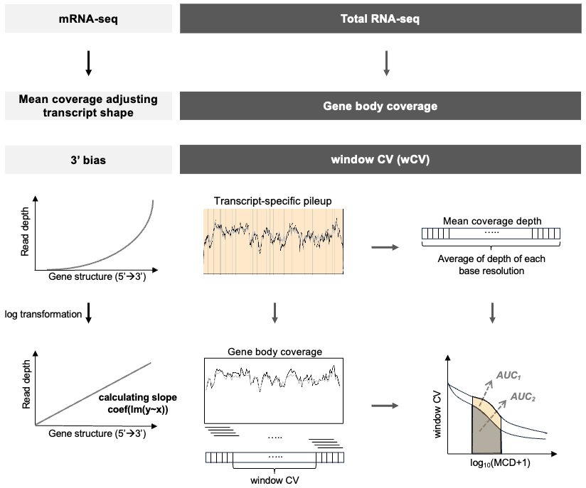
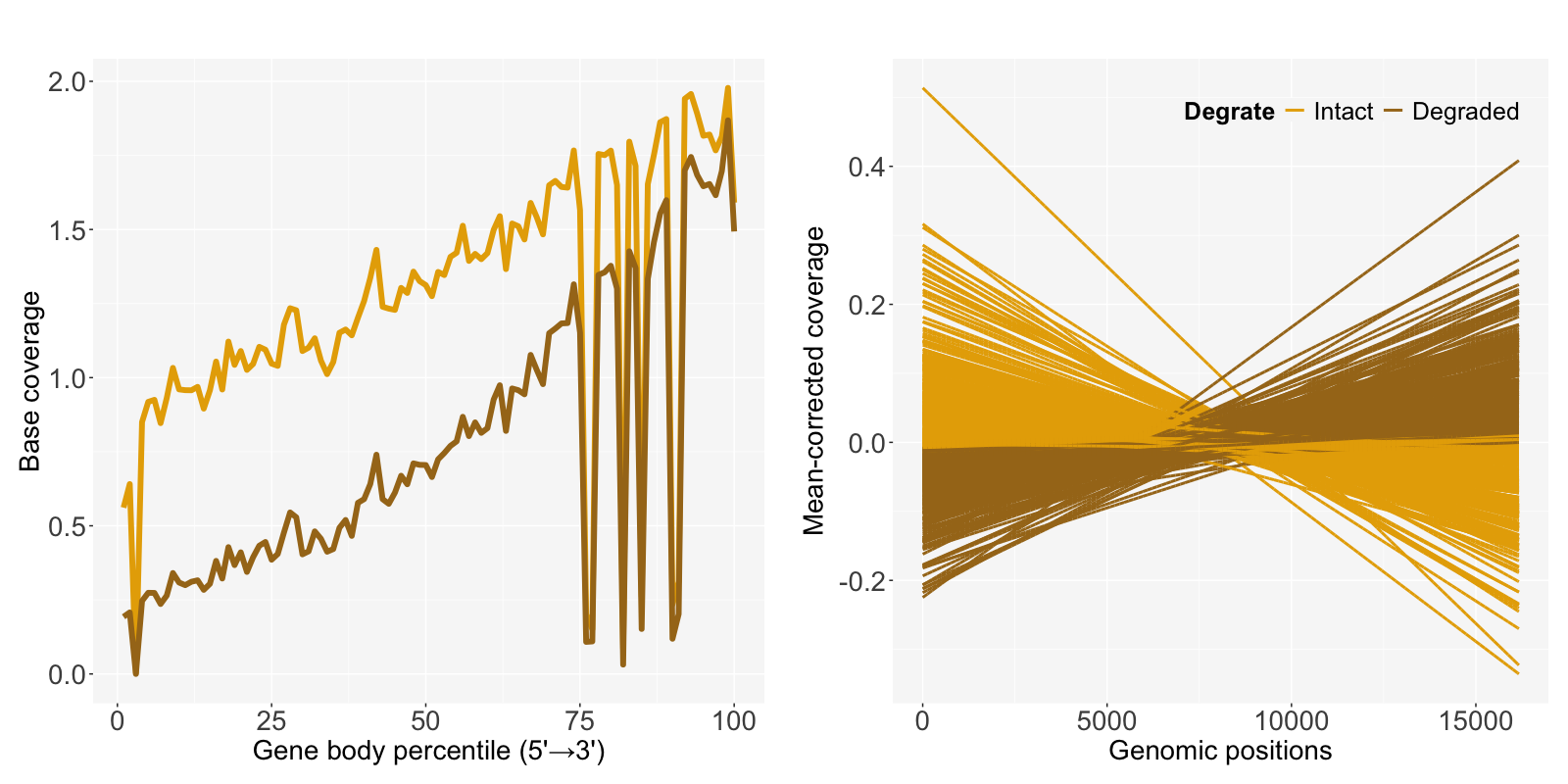
Choi et al. (2021)¹ suggested decay rate by the mean-corrected slope of log-transformed data to measure the extent of degradation and identify degraded samples in mRNA-seq. SCISSOR::decay.rate.hy calculates slopes and decay rates for all samples with exon-only coverage pileupData from get_pileupExon function.

library(SCISSOR)

d <- dim(pileupData)[1]
data.process <- SCISSOR::process_pileup(pileupData=pileupData, Ranges=exonRanges,
                                        logshiftVal=10, plotNormalization=F)
decayRate <- SCISSOR::decay.rate.hy(Data=data.process$normalizedData)$slope*d

In case of a long gene FAT1 with fresh frozen and mRNA-seq (FFM) 589 samples from TCGA-LUAD, total length d is 16,167 and slope is calculated by fitting a linear regression of genomic positions and the mean-corrected coverage. Degrate is defined as Intact or Degraded based on the median of decayRate to compare the degradation effect in base coverage. The degraded samples having relatively larger slopes show lower coverage.

In our package, we propose a novel approach sample quality index (SQI) based on window coefficient of variation (wCV) to assess RNA-seq data quality for total RNA-seq and FFPE samples.

5.2 Sample quality index

A mean coverage depth (MCD) and wCV can be calculated from the get_MCD and get_wCV functions. To adjust the effect of low base coverage to CV, we consider wCV within a restricted range of MCD. Both functions return the same dimension of a matrix, which is the number of genes $\times$ the number of samples.

MCD.mat = get_MCD(genelist, pileupPath, sampleInfo)
wCV.mat = get_wCV(genelist, pileupPath, sampleInfo, rnum=100, method=1, winSize=20, egPct=10)

The get_SQI function gives the AUC of the fitted lines in the regression of wCV and log transformed MCD, and normalizes it using projection depth (PD)². Finally, we can determine the quality of the samples by defining them as Bad if PD>3. Nineteen out of 171 samples are classified as bad quality samples. The SQI plot shows the distribution of AUC and PD and the shape of the regression by sample quality.

result = get_SQI(MCD=MCD.mat, wCV=wCV.mat, rstPct=20, obsPct=50)
auc.vec <- result$auc.vec
# table(auc.vec$SQI)

plot_SQI(SQIresult=result)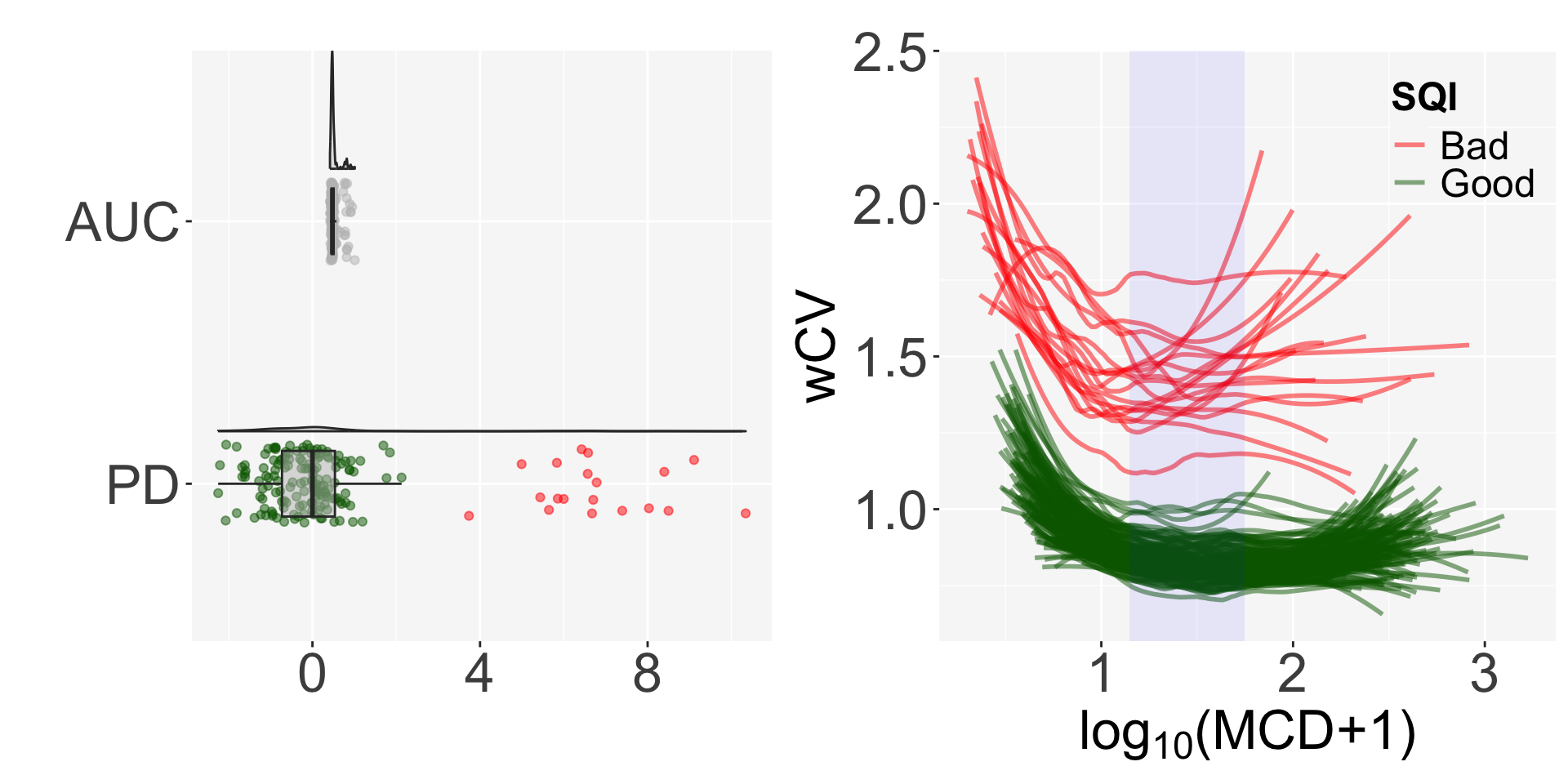

5.3 Updated gene body coverage

The gene body coverage plots in gene body coverage chapter can be updated after removing bad samples using the plot_GBCg function. The coverage patterns become much more stable, especially in the long genes.

GBCg0 = plot_GBCg(stat=2, plot=TRUE, sampleInfo, GBCresult=GBC0, auc.vec=result$auc.vec)
GBCg5 = plot_GBCg(stat=2, plot=TRUE, sampleInfo, GBCresult=GBC5, auc.vec=result$auc.vec)

pg0 <- GBCg0$plotRI +
  coord_cartesian(ylim=c(0, 0.017)) +
  ggtitle("0~5 kb")
pg5 <- GBCg5$plotRI +
  coord_cartesian(ylim=c(0, 0.017)) +
  ggtitle("5+ kb")

ggpubr::ggarrange(pg0, pg5, common.legend=TRUE, legend="bottom", nrow=1)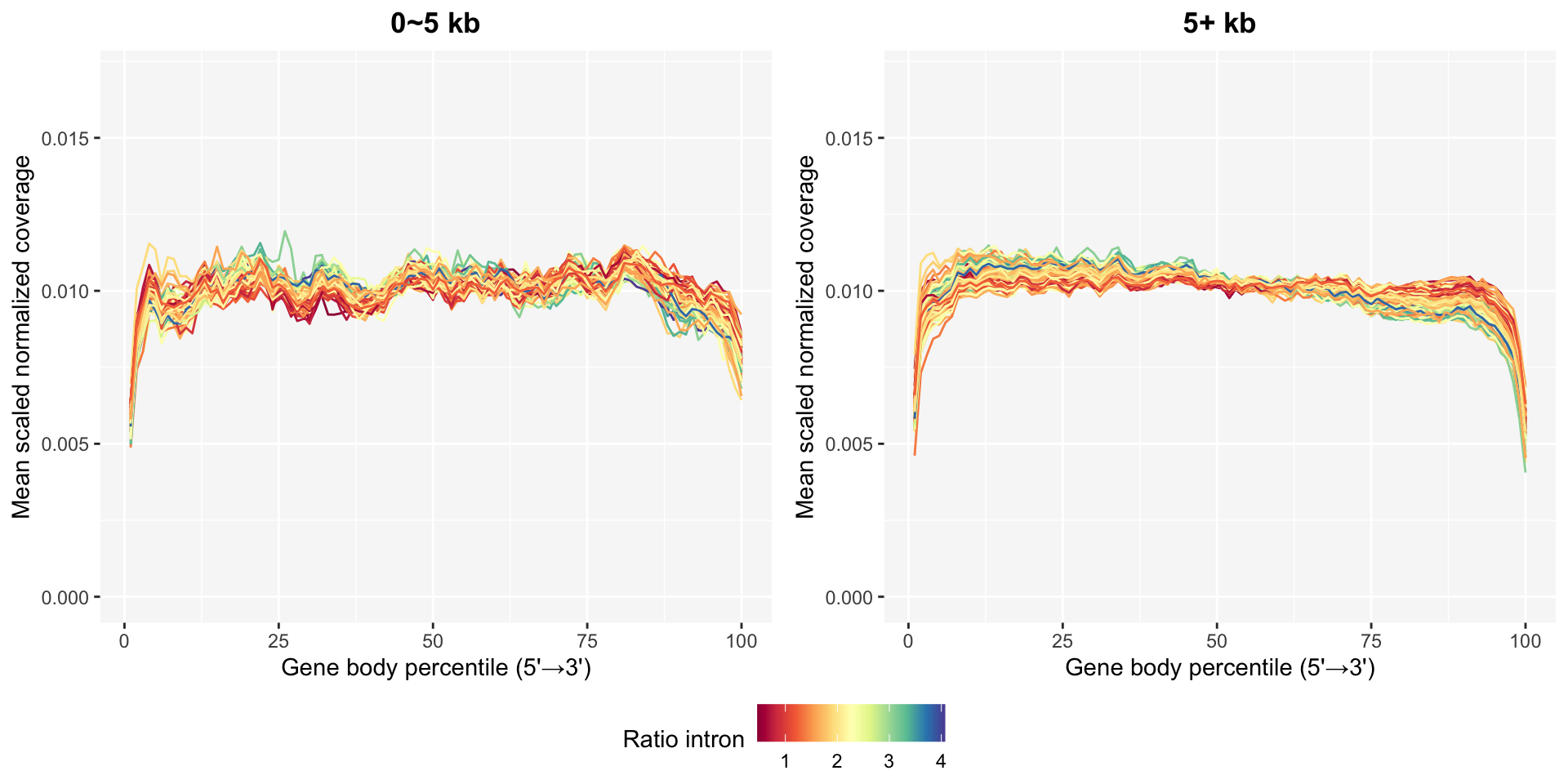

This function provides a continuous legend option to select such as ratio intron or PD for the line color.

pg0 <- GBCg0$plotPD +
  coord_cartesian(ylim=c(0, 0.017)) +
  ggtitle("0~5 kb")
pg5 <- GBCg5$plotPD +
  coord_cartesian(ylim=c(0, 0.017)) +
  ggtitle("5+ kb")

ggpubr::ggarrange(pg0, pg5, common.legend=TRUE, legend="bottom", nrow=1)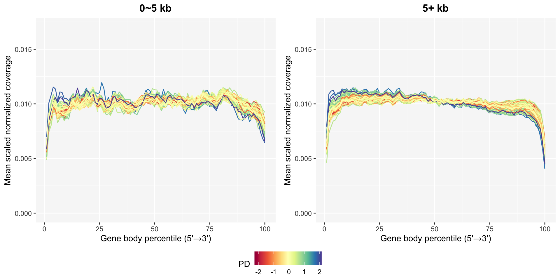

---

1. Choi, H.Y., Jo, H., Zhao, X. et al. SCISSOR: a framework for identifying structural changes in RNA transcripts. Nat Commun 12, 286 (2021). https://doi.org/10.1038/s41467-020-20593-3↩︎

2. Choi, H. (2018). Scissor for finding outliers in RNA-seq. https://doi.org/10.17615/dv2e-7a29↩︎