library(modsem)9 plotting interaction effects
10 Plotting interaction effects
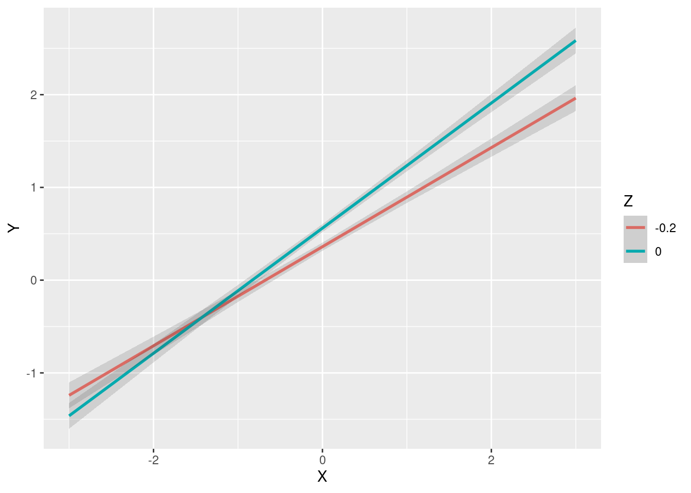
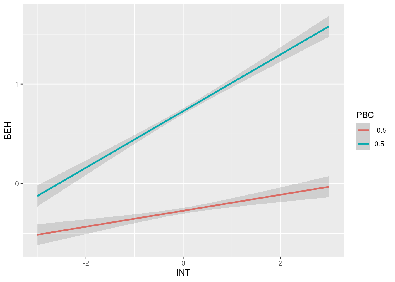
Interaction effects can be plotted using the included plot_interaction function. This function takes a fitted model object and the names of the two variables that are interacting. The function will plot the interaction effect of the two variables. The x-variable is plotted on the x-axis and the y-variable is plotted on the y-axis. And the z-variable decides at what points of z the effect of x on y is plotted. The function will also plot the 95% confidence interval of the interaction effect.
Here we can see a simple example using the double centering approach.
m1 <- "
# Outer Model
  X =~ x1
  X =~ x2 + x3
  Z =~ z1 + z2 + z3
  Y =~ y1 + y2 + y3

# Inner model
  Y ~ X + Z + X:Z
"
est1 <- modsem(m1, data = oneInt)
plot_interaction("X", "Z", "Y", "X:Z", -3:3, c(-0.2, 0), est1)
Here we can see a different example using the LMS approach, in the theory of planned behavior model.
tpb <- "
# Outer Model (Based on Hagger et al., 2007)
  ATT =~ att1 + att2 + att3 + att4 + att5
  SN =~ sn1 + sn2
  PBC =~ pbc1 + pbc2 + pbc3
  INT =~ int1 + int2 + int3
  BEH =~ b1 + b2

# Inner Model (Based on Steinmetz et al., 2011)
  INT ~ ATT + SN + PBC
  BEH ~ INT + PBC
  BEH ~ PBC:INT
"

est2 <- modsem(tpb, TPB, method = "lms")
#> Warning: It is recommended that you have at least 32 nodes for interaction
#> effects between exogenous and endogenous variables in the lms approach 'nodes =
#> 24'
plot_interaction(x = "INT", z = "PBC", y = "BEH", xz = "PBC:INT",
                 vals_z = c(-0.5, 0.5), model = est2)