Chapter3 GAMA101- Mathematics for Computer and Information Science-1

Course Objective: This course is designed as an entry level course to Computer and Informations Science. Upon successful completion of this course the student can use calculus as effective tool for analysis.

3.1 Module-1 Single Variable Calculus and its applications in Computer Science

Syllabus Content: Limits of Function Values, The Limit Laws, Continuous Functions, Rates of Change, Second- and Higher-Order Derivatives, Instantaneous Rates of Change, Derivative as a Function , Chain Rule, Implicit Differentiation, Tangents and Normal Lines, Linearization, Concavity. Reference text & Sections: (Thomas Jr et al. 2014),Relevant topics from sections 2.2, 2.5, 3.1, 3.2, 3.3, 3.4, 3.6,3.7, 3.9, 4.4

3.1.1 Instanteneous Average Throughput of a Network using limit

Suppose we want to calculate the average throughput (data transfer rate) of a network over a week. The throughput \(D\) (in megabits per second, Mbps) is recorded periodically:

• Monday: \(D = 100\) Mbps
• Tuesday: \(D = 110\) Mbps
• Wednesday: \(D = 120\) Mbps
• Thursday: \(D = 115\) Mbps
• Friday: \(D = 105\) Mbps
• Saturday: \(D = 108\) Mbps
• Sunday: \(D = 112\) Mbps

To find the average throughput over the week, we use the standard formula for average: \[ \text{Average Throughput} = \frac{D_{\text{Mon}} + D_{\text{Tue}} + D_{\text{Wed}} + D_{\text{Thu}} + D_{\text{Fri}} + D_{\text{Sat}} + D_{\text{Sun}}}{7} \]

Let’s calculate this:

1. Sum of Throughputs: \[ D_{\text{total}} = 100 + 110 + 120 + 115 + 105 + 108 + 112 = 770 \text{ Mbps} \]

2. Average Throughput: \[ \text{Average Throughput} = \frac{770}{7} \approx 110 \text{ Mbps} \]

Now, let’s formulate and interpret this in terms of a limit in computer science:

Limit Interpretation

Suppose we want to estimate the average throughput if we measured it continuously rather than periodically, approaching continuous monitoring: \[ \lim_{\Delta t \to 0} \frac{\sum D(t)}{n} \]

Here, \(\Delta t\) represents the time interval (approaching zero), \(D(t)\) is the throughput at time \(t\), and \(n\) is the number of intervals.

Interpretation

As \(\Delta t\) (the time interval) approaches zero, the average throughput calculated for smaller and smaller time intervals (like per second instead of per day) would approach the continuous average throughput we would theoretically obtain if we could monitor throughput continuously.

This example demonstrates how limits can be applied in computer science to understand data processing rates or system performance as we consider finer and finer time resolutions (approaching continuous monitoring). It aligns with concepts like real-time data processing, system performance analysis, and network optimization, where understanding behavior as variables approach specific conditions (like time intervals approaching zero) is crucial.

3.2 Refreshing knowledge

• Main points to be highlighted along with the formal definition
  1. The limit is a value one expect that function would have at the point \(x=a\), based on the values of that function at close vicinity of \(x=a\), but regardless of the value of \(f(x)\) at \(x=a\), if \(f(a)\) is defined at all. Use the link https://en.wikipedia.org/wiki/Limit_of_a_function#/media/File:Epsilon-delta_limit.svg for geometrical explanation for a better understanding.
  2. For the existence of limit at \(x=a\), \(f(a^+)=f(a^-)\). Use this property geometrically to check existence of limit at \(x=0\) of the unit step function and similar examples from the text book.

An interesting video session is available at:

3.3 Limit of a Function

3.3.1 Understanding Limits of a Function

The concept of a limit is essential for studying the local behavior of a function near a specified point. It helps us understand how a function behaves as the input value approaches a particular point from both the left and the right.

3.3.1.1 Identity Function \(f(x) = x\)

For the identity function \(f(x) = x\):

• Left-hand limit as \(x\) approaches \(a\): \[ \lim_{{x \to a^-}} x = \lim_{{h \to 0}} (a - h) = a \]
• Right-hand limit as \(x\) approaches \(a\): \[ \lim_{{x \to a^+}} x = \lim_{{h \to 0}} (a + h) = a \]

Python Visualization:

import numpy as np
import matplotlib.pyplot as plt

# Identity function
def f(x):
    return x

a = 2  # Point to approach
h_values = np.linspace(0.01, 1, 100)

# Left-hand limit
left_hand_limit = f(a - h_values)
# Right-hand limit
right_hand_limit = f(a + h_values)

plt.figure(figsize=(10, 6))
plt.plot(a - h_values, left_hand_limit, label='Left-hand limit (a-h)', color='blue')
plt.plot(a + h_values, right_hand_limit, label='Right-hand limit (a+h)', color='red')
plt.axvline(x=a, color='black', linestyle='--')
plt.scatter([a], [f(a)], color='green', zorder=5)
plt.text(a, f(a), '  f(a)', fontsize=12, verticalalignment='bottom')

plt.xlabel('x')
plt.ylabel('f(x)')
plt.title('Left-hand and Right-hand Limits of f(x) = x as x approaches a')
plt.legend()
plt.grid(True)
plt.show()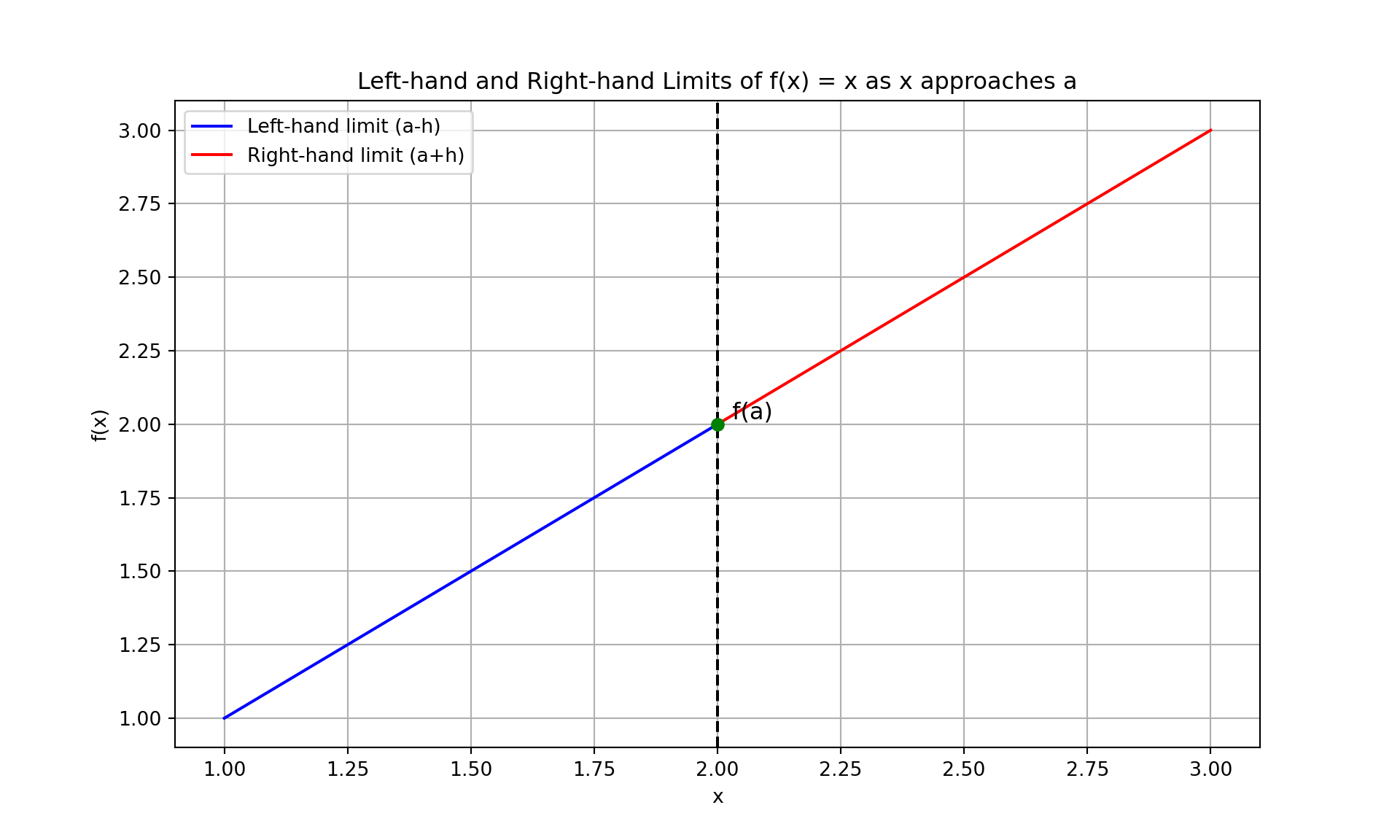

3.3.1.2 Constant Function \(f(x) = c\)

For a constant function \(f(x) = c\):

• Left-hand limit as \(x\) approaches \(a\): \[ \lim_{{x \to a^-}} c = c \]
• Right-hand limit as \(x\) approaches \(a\): \[ \lim_{{x \to a^+}} c = c \]

Python Visualization:

import numpy as np
import matplotlib.pyplot as plt

# Constant function
def f(x):
    return np.full_like(x, 5)  # Constant value

a = 3  # Point to approach
h_values = np.linspace(0.01, 1, 100)

# Left-hand limit
left_hand_limit = f(a - h_values)
# Right-hand limit
right_hand_limit = f(a + h_values)

x_range = np.linspace(a - 2, a + 2, 400)
y_range = f(x_range)

plt.figure(figsize=(10, 6))
plt.plot(x_range, y_range, label='f(x) = 5', color='blue')
plt.axvline(x=a, color='black', linestyle='--')
plt.scatter([a], [f(a)], color='green', zorder=5)
plt.text(a, f(a), '  f(a)', fontsize=12, verticalalignment='bottom')

plt.xlabel('x')
plt.ylabel('f(x)')
plt.title('Left-hand and Right-hand Limits of f(x) = 5 as x approaches a')
plt.legend()
plt.grid(True)
plt.show()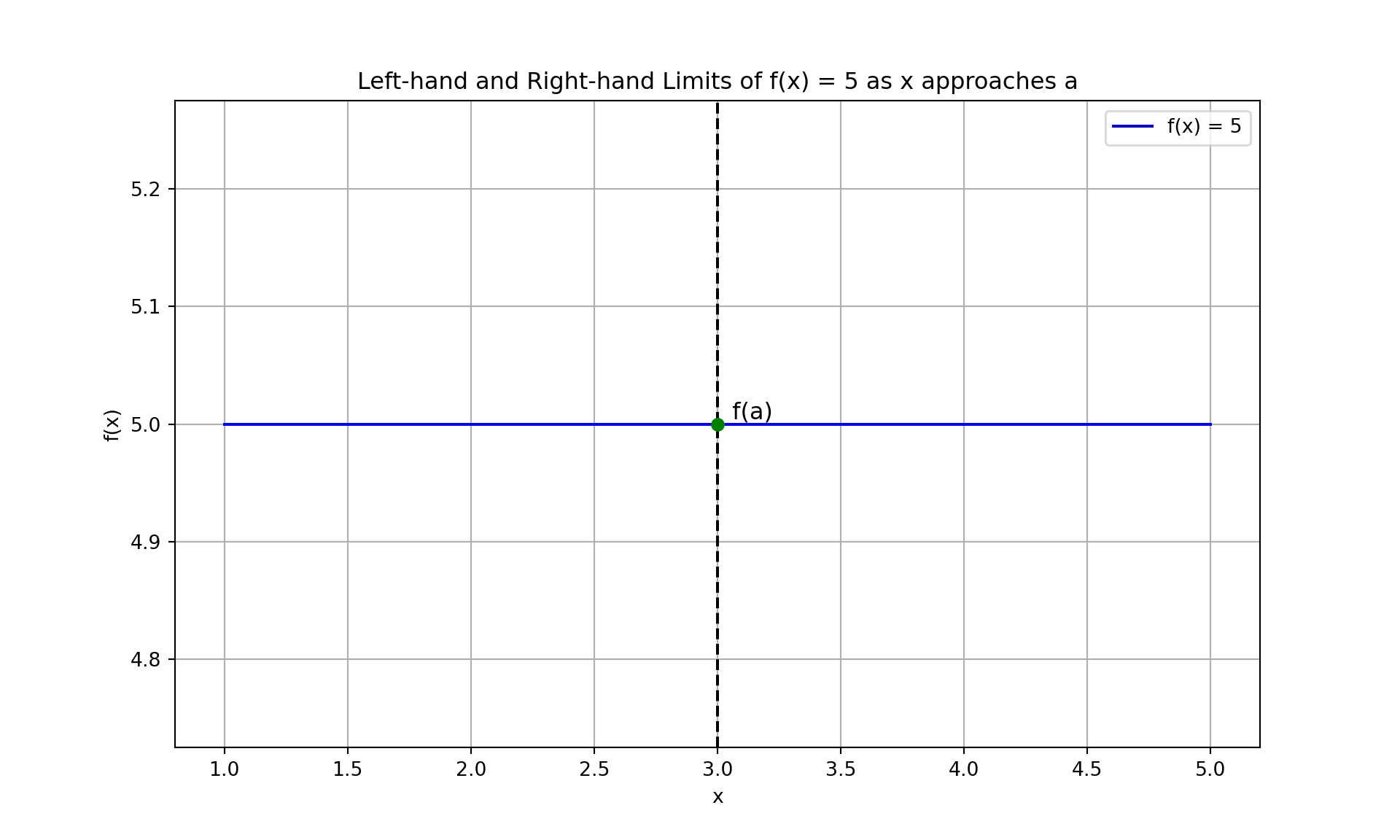

3.3.1.3 Unit Step Function \(u(x)\)

The unit step function \(u(x)\) is defined as: \[ u(x) = \begin{cases} 0 & \text{if } x < 0 \\ 1 & \text{if } x \geq 0 \end{cases} \]

• Left-hand limit as \(x\) approaches 0: \[ \lim_{{x \to 0^-}} u(x) = \lim_{{h \to 0}} u(-h) = 0 \]
• Right-hand limit as \(x\) approaches 0: \[ \lim_{{x \to 0^+}} u(x) = \lim_{{h \to 0}} u(h) = 1 \]

Python Visualization:

import numpy as np
import matplotlib.pyplot as plt

# Unit step function
def u(x):
    return np.where(x < 0, 0, 1)

a = 0  # Point to approach
h_values = np.linspace(0.01, 1, 100)

# Left-hand limit
left_hand_limit = u(a - h_values)
# Right-hand limit
right_hand_limit = u(a + h_values)

plt.figure(figsize=(10, 6))
plt.plot(a - h_values, left_hand_limit, label='Left-hand limit (a-h)', color='blue')
plt.plot(a + h_values, right_hand_limit, label='Right-hand limit (a+h)', color='red')
plt.axvline(x=a, color='black', linestyle='--')
plt.scatter([a], [u(a)], color='green', zorder=5)
plt.text(a, u(a), '  u(a)', fontsize=12, verticalalignment='bottom')

plt.xlabel('x')
plt.ylabel('u(x)')
plt.title('Left-hand and Right-hand Limits of Unit Step Function as x approaches 0')
plt.legend()
plt.grid(True)
plt.show()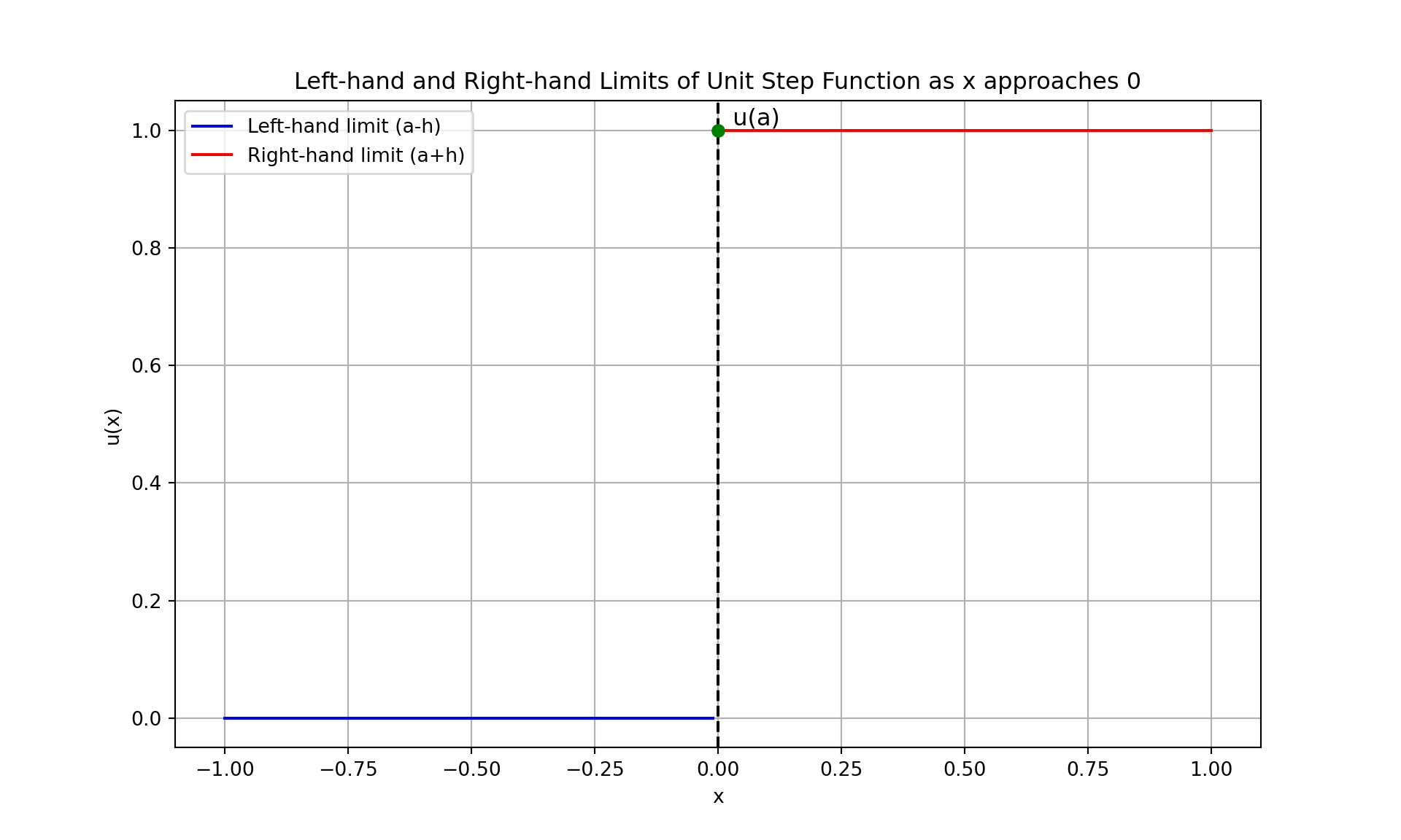

3.3.1.4 Signum Function \(\text{sgn}(x)\)

The signum function \(\text{sgn}(x)\) is defined as: \[ \text{sgn}(x) = \begin{cases} -1 & \text{if } x < 0 \\ 0 & \text{if } x = 0 \\ 1 & \text{if } x > 0 \end{cases} \]

• Left-hand limit as \(x\) approaches 0: \[ \lim_{{x \to 0^-}} \text{sgn}(x) = \lim_{{h \to 0}} \text{sgn}(-h) = -1 \]
• Right-hand limit as \(x\) approaches 0: \[ \lim_{{x \to 0^+}} \text{sgn}(x) = \lim_{{h \to 0}} \text{sgn}(h) = 1 \]

Python Visualization:

import numpy as np
import matplotlib.pyplot as plt

# Signum function
def sgn(x):
    return np.where(x < 0, -1, np.where(x > 0, 1, 0))

a = 0  # Point to approach
h_values = np.linspace(0.01, 1, 100)

# Left-hand limit
left_hand_limit = sgn(a - h_values)
# Right-hand limit
right_hand_limit = sgn(a + h_values)

plt.figure(figsize=(10, 6))
plt.plot(a - h_values, left_hand_limit, label='Left-hand limit (a-h)', color='blue')
plt.plot(a + h_values, right_hand_limit, label='Right-hand limit (a+h)', color='red')
plt.axvline(x=a, color='black', linestyle='--')
plt.scatter([a], [sgn(a)], color='green', zorder=5)
plt.text(a, sgn(a), '  sgn(a)', fontsize=12, verticalalignment='bottom')

plt.xlabel('x')
plt.ylabel('sgn(x)')
plt.title('Left-hand and Right-hand Limits of Signum Function as x approaches 0')
plt.legend()
plt.grid(True)
plt.show()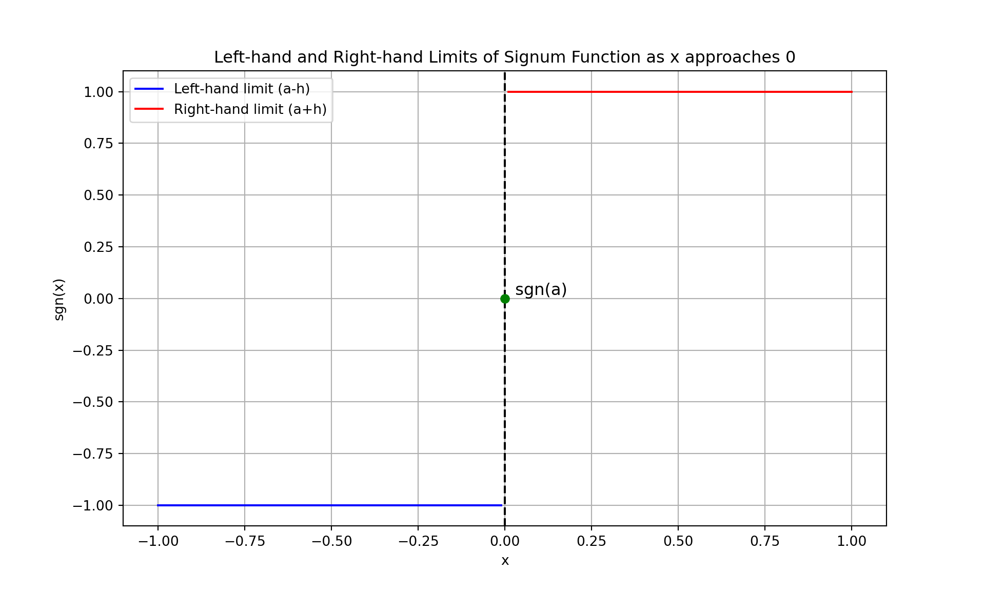

3.3.1.5 Sigmoid Function \(\sigma(x)\)

The sigmoid function \(\sigma(x)\) is defined as: \[ \sigma(x) = \frac{1}{1 + e^{-x}} \]

• Left-hand limit as \(x\) approaches 0: \[ \lim_{{x \to 0^-}} \sigma(x) = \frac{1}{1 + e^{-0}} = \frac{1}{2} \]
• Right-hand limit as \(x\) approaches 0: \[ \lim_{{x \to 0^+}} \sigma(x) = \frac{1}{1 + e^{0}} = \frac{1}{2} \]

Python Visualization:

import numpy as np
import matplotlib.pyplot as plt

# Sigmoid function
def sigmoid(x):
    return 1 / (1 + np.exp(-x))

a = 0  # Point to approach
h_values = np.linspace(0.01, 1, 100)

# Left-hand limit
left_hand_limit = sigmoid(a - h_values)
# Right-hand limit
right_hand_limit = sigmoid(a + h_values)

x_range = np.linspace(a - 5, a + 5, 400)
y_range = sigmoid(x_range)

plt.figure(figsize=(10, 6))
plt.plot(x_range, y_range, label='σ(x) = 1 / (1 + e^(-x))', color='blue')
plt.plot(a - h_values, left_hand_limit, label='Left-hand limit (a-h)', color='yellow')
plt.plot(a + h_values, right_hand_limit, label='Right-hand limit (a+h)', color='red')
plt.axvline(x=a, color='black', linestyle='--')
plt.scatter([a], [sigmoid(a)], color='green', zorder=5)
plt.text(a, sigmoid(a), '  σ(a)', fontsize=12, verticalalignment='bottom')

plt.xlabel('x')
plt.ylabel('σ(x)')
plt.title('Left-hand and Right-hand Limits of Sigmoid Function as x approaches 0')
plt.legend()
plt.grid(True)
plt.show()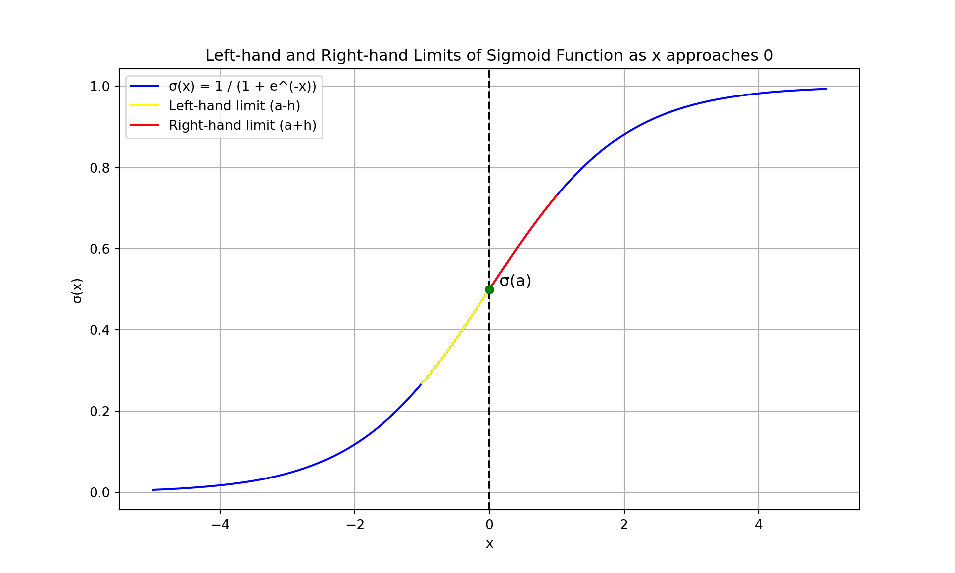

3.3.1.6 Piecewise Function \(f(x)\)

The piecewise function \(f(x)\) is defined as: \[ f(x) = \begin{cases} \sin\left(\frac{1}{x}\right) & \text{if } x > 0 \\ 0 & \text{if } x \leq 0 \end{cases} \]

• Left-hand limit as \(x\) approaches 0: \[ \lim_{{x \to 0^-}} f(x) = 0 \]
• Right-hand limit as \(x\) approaches 0: \[ \lim_{{x \to 0^+}} f(x) = \text{Does not exist (oscillates)} \]

Python Visualization:

import numpy as np
import matplotlib.pyplot as plt

# Piecewise function
def f(x):
    # Avoid division by zero by only applying the function where x is positive
    return np.where(x > 0, np.sin(1 / x), 0)

a = 0  # Point to approach
h_values = np.linspace(0.01, 0.1, 100)

# Left-hand limit (x <= 0)
x_negative_h_values = -h_values
left_hand_limit = f(x_negative_h_values)

# Right-hand limit (x > 0)
x_positive_h_values = h_values
right_hand_limit = f(x_positive_h_values)

x_range = np.linspace(a - 0.2, a + 0.2, 400)
y_range = f(x_range)

plt.figure(figsize=(10, 6))
plt.plot(x_range, y_range, label='f(x) = sin(1/x) for x > 0, 0 for x <= 0', color='blue')
plt.plot(a - h_values, left_hand_limit, label='Left-hand limit (a-h)', color='yellow')
plt.plot(a + h_values, right_hand_limit, label='Right-hand limit (a+h)', color='red')
plt.axvline(x=a, color='black', linestyle='--')
#plt.scatter([a], [f(a)], color='green', zorder=5)
#plt.text(a, f(a), '  f(a)', fontsize=12, verticalalignment='bottom')

plt.xlabel('x')
plt.ylabel('f(x)')
plt.title('Left-hand and Right-hand Limits of Piecewise Function as x approaches 0')
plt.legend()
plt.grid(True)
plt.show()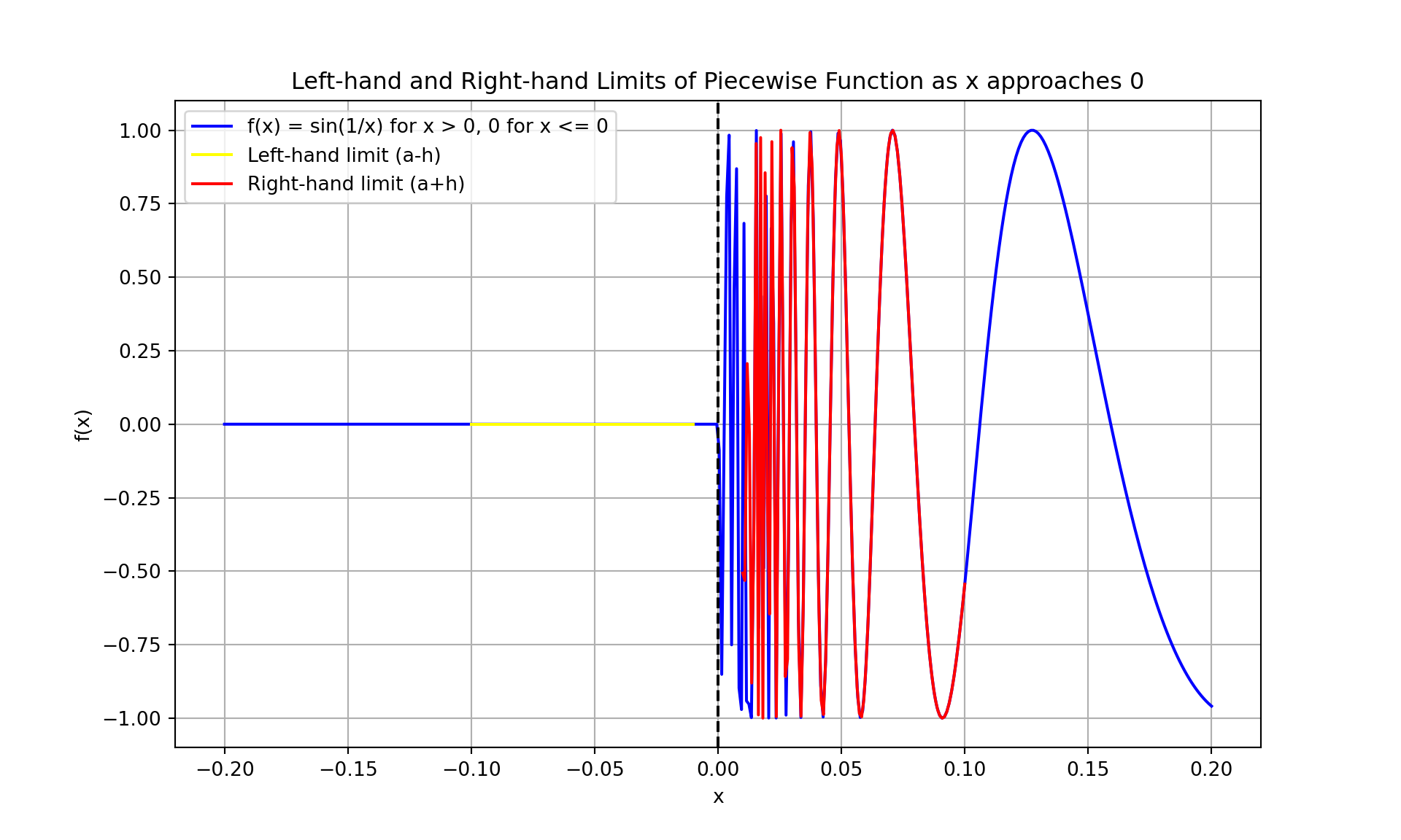

3.3.1.7 Takeaway

In this introductory session on limits, we explored how single-variable functions behave as they approach a specific point from both sides. Here are the key takeaways:

• Definition of Limits: The limit of a function at a point provides insight into the function’s behavior as it approaches that point from both directions. Specifically:
  • Left-hand limit: The value the function approaches as the input approaches the point from the left.
  • Right-hand limit: The value the function approaches as the input approaches the point from the right.
• Stability in Behavior: A function is considered stable at a point if the left-hand limit and the right-hand limit are equal. This implies that:
  • The function approaches the same value from both sides of the point.
  • The function has a well-defined limit at that point.

3.3.1.8 Examples

1. Constant Function:
   • For \(f(x) = c\), the left-hand limit and the right-hand limit are both \(c\), demonstrating stability.
2. Unit Step Function:
   • For \(u(x)\), the left-hand limit as \(x\) approaches 0 is 0, while the right-hand limit is 1, indicating a discontinuity at \(x = 0\).
3. Sigmoid Function:
   • For \(\sigma(x) = \frac{1}{1 + e^{-x}}\), both the left-hand limit and the right-hand limit as \(x\) approaches 0 are \(\frac{1}{2}\), showing stability.
4. Piecewise Function \(f(x)\):
   • For \(f(x) = \sin\left(\frac{1}{x}\right)\) for \(x > 0\) and \(0\) for \(x \leq 0\), the left-hand limit is 0, and the right-hand limit does not exist due to oscillation, showing instability.

By analyzing these examples, we observe that stability at a point is characterized by the equality of the left-hand and right-hand limits. When these limits are equal, the function is said to be continuous at that point. When they are not equal or the limit does not exist, the function may exhibit discontinuities or oscillatory behavior.

Understanding limits helps in analyzing and predicting the behavior of functions in various contexts, including computer science, where stability and continuity can be crucial in algorithms and system behaviors.

3.3.2 Practice Problems

Solving Limits of Functions - Thomas Calculus Section 2.2

1. Problem: Find the limit of the function \(f(x) = 3x^2 - 2x + 1\) as \(x\) approaches 2.

Solution: \[ \lim_{{x \to 2}} (3x^2 - 2x + 1) = 3(2)^2 - 2(2) + 1 = 12 - 4 + 1 = 9 \]

• Left-hand limit: \(\lim\limits_{{x \to 2^-}} (3x^2 - 2x + 1) = 9\)

• Right-hand limit: \(\lim\limits_{{x \to 2^+}} (3x^2 - 2x + 1) = 9\)

2. Problem: Find the limit of the function \(f(x) = \sqrt{x + 4}\) as \(x\) approaches 1.

Solution: \[ \lim_{{x \to 1}} \sqrt{x + 4} = \sqrt{1 + 4} = \sqrt{5} \]

• Left-hand limit: \(\lim\limits_{{x \to 1^-}} \sqrt{x + 4} = \sqrt{5}\)

• Right-hand limit: \(\lim\limits_{{x \to 1^+}} \sqrt{x + 4} = \sqrt{5}\)

3. Problem: Find the limit of the function \(f(x) = \frac{x^2 - 1}{x - 1}\) as \(x\) approaches 1.

Solution: First, simplify the function: \[ \frac{x^2 - 1}{x - 1} = \frac{(x - 1)(x + 1)}{x - 1} = x + 1 \quad \text{for } x \neq 1 \] Thus, \[ \lim_{{x \to 1}} \frac{x^2 - 1}{x - 1} = \lim_{{x \to 1}} (x + 1) = 2 \]

• Left-hand limit: \(\lim\limits_{{x \to 1^-}} \frac{x^2 - 1}{x - 1} = 2\)

• Right-hand limit: \(\lim\limits_{{x \to 1^+}} \frac{x^2 - 1}{x - 1} = 2\)

4. Problem: Find the limit of the function \(f(x) = \frac{\sin(x)}{x}\) as \(x\) approaches 0.

Solution: Use the fact that \(\lim\limits_{{x \to 0}} \frac{\sin(x)}{x} = 1\): \[ \lim_{{x \to 0}} \frac{\sin(x)}{x} = 1 \]

• Left-hand limit: \(\lim_{{x \to 0^-}} \frac{\sin(x)}{x} = 1\)
• Right-hand limit: \(\lim_{{x \to 0^+}} \frac{\sin(x)}{x} = 1\)

5. Problem: Find the limit of the function \(f(x) = \frac{e^x - 1}{x}\) as \(x\) approaches 0.

Solution: Apply L’Hôpital’s rule, which is used when the limit is of the form \(\frac{0}{0}\): \[ \lim_{{x \to 0}} \frac{e^x - 1}{x} = \lim_{{x \to 0}} \frac{e^x}{1} = e^0 = 1 \]

• Left-hand limit: \(\lim\limits_{{x \to 0^-}} \frac{e^x - 1}{x} = 1\)

• Right-hand limit: \(\lim\limits_{{x \to 0^+}} \frac{e^x - 1}{x} = 1\)

6. Problem: Find the limit of the function \(f(x) = \frac{\ln(x)}{x - 1}\) as \(x\) approaches 1.

Solution: Apply L’Hôpital’s rule: \[ \lim_{{x \to 1}} \frac{\ln(x)}{x - 1} = \lim_{{x \to 1}} \frac{\frac{d}{dx}[\ln(x)]}{\frac{d}{dx}[x - 1]} = \lim_{{x \to 1}} \frac{\frac{1}{x}}{1} = \frac{1}{1} = 1 \]

• Left-hand limit: \(\lim\limits_{{x \to 1^-}} \frac{\ln(x)}{x - 1} = 1\)

• Right-hand limit: \(\lim\limits_{{x \to 1^+}} \frac{\ln(x)}{x - 1} = 1\)

7. Problem: Find the limit of the function \(f(x) = \frac{x^3 - 8}{x - 2}\) as \(x\) approaches 2.

Solution: First, simplify the function using polynomial division or factoring: \[ \frac{x^3 - 8}{x - 2} = \frac{(x - 2)(x^2 + 2x + 4)}{x - 2} = x^2 + 2x + 4 \quad \text{for } x \neq 2 \] Thus, \[ \lim_{{x \to 2}} \frac{x^3 - 8}{x - 2} = \lim_{{x \to 2}} (x^2 + 2x + 4) = 4 + 4 + 4 = 12 \]

• Left-hand limit: \(\lim\limits_{{x \to 2^-}} \frac{x^3 - 8}{x - 2} = 12\)

• Right-hand limit: \(\lim\limits_{{x \to 2^+}} \frac{x^3 - 8}{x - 2} = 12\)

8. Problem: Find the limit of the function \(f(x) = \frac{\tan(x)}{x}\) as \(x\) approaches 0.

Solution: Use the fact that \(\lim_{{x \to 0}} \frac{\tan(x)}{x} = 1\): \[ \lim_{{x \to 0}} \frac{\tan(x)}{x} = 1 \]

• Left-hand limit: \(\lim\limits_{{x \to 0^-}} \frac{\tan(x)}{x} = 1\)

• Right-hand limit: \(\lim\limits_{{x \to 0^+}} \frac{\tan(x)}{x} = 1\)

9. Problem: Find the limit of the function \(f(x) = \frac{x^2 - 4}{x^2 - x - 6}\) as \(x\) approaches 3.

Solution: First, simplify the function by factoring: \[ \frac{x^2 - 4}{x^2 - x - 6} = \frac{(x - 2)(x + 2)}{(x - 3)(x + 2)} = \frac{x - 2}{x - 3} \quad \text{for } x \neq 3 \] Thus, \[ \lim_{{x \to 3}} \frac{x^2 - 4}{x^2 - x - 6} = \lim_{{x \to 3}} \frac{x - 2}{x - 3} = \frac{3 - 2}{3 - 3} = \text{Undefined (asymptote)} \]

• Left-hand limit: \(\lim\limits_{{x \to 3^-}} \frac{x^2 - 4}{x^2 - x - 6} = -\infty\)

• Right-hand limit: \(\lim\limits_{{x \to 3^+}} \frac{x^2 - 4}{x^2 - x - 6} = +\infty\)

10. Problem: Find the limit of the function \(f(x) = \frac{e^{2x} - e^x}{x}\) as \(x\) approaches 0.

Solution: Apply L’Hôpital’s rule: \[ \lim_{{x \to 0}} \frac{e^{2x} - e^x}{x} = \lim_{{x \to 0}} \frac{2e^{2x} - e^x}{1} = 2e^0 - e^0 = 2 - 1 = 1 \]

• Left-hand limit: \(\lim\limits_{{x \to 0^-}} \frac{e^{2x} - e^x}{x} = 1\)

• Right-hand limit: \(\lim\limits_{{x \to 0^+}} \frac{e^{2x} - e^x}{x} = 1\)

3.3.3 Limit laws

Serial No.	Law	Description	Formula
1	Constant Law	If \(c\) is a constant, then:	\[ \lim_{{x \to a}} c = c \]
2	Identity Law	If \(f(x) = x\), then:	\[ \lim_{{x \to a}} x = a \]
3	Sum Law	If \(\lim_{{x \to a}} f(x) = L\) and \(\lim_{{x \to a}} g(x) = M\), then:	\[ \lim_{{x \to a}} [f(x) + g(x)] = L + M \]
4	Difference Law	If \(\lim_{{x \to a}} f(x) = L\) and \(\lim_{{x \to a}} g(x) = M\), then:	\[ \lim_{{x \to a}} [f(x) - g(x)] = L - M \]
5	Product Law	If \(\lim_{{x \to a}} f(x) = L\) and \(\lim_{{x \to a}} g(x) = M\), then:	\[ \lim_{{x \to a}} [f(x) \cdot g(x)] = L \cdot M \]
6	Quotient Law	If \(\lim_{{x \to a}} f(x) = L\) and \(\lim_{{x \to a}} g(x) = M\), and \(M \neq 0\), then:	\[ \lim_{{x \to a}} \frac{f(x)}{g(x)} = \frac{L}{M} \]
7	Power Law	If \(\lim_{{x \to a}} f(x) = L\) and \(n\) is a positive integer, then:	\[ \lim_{{x \to a}} [f(x)]^n = L^n \]
8	Root Law	If \(\lim_{{x \to a}} f(x) = L\) and \(n\) is a positive integer, then:	\[ \lim_{{x \to a}} \sqrt[n]{f(x)} = \sqrt[n]{L} \]
9	Composite Function Law	If \(\lim_{{x \to a}} f(x) = L\) and \(\lim_{{x \to L}} g(x) = M\), then:	\[ \lim_{{x \to a}} g(f(x)) = M \]
10	Limit of a Constant Multiple	If \(\lim_{{x \to a}} f(x) = L\) and \(c\) is a constant, then:	\[ \lim_{{x \to a}} [c \cdot f(x)] = c \cdot L \]
11	Limit of a Function Raised to a Power	If \(\lim_{{x \to a}} f(x) = L\) and \(n\) is a positive integer, then:	\[ \lim_{{x \to a}} [f(x)]^n = L^n \]

3.3.4 Limit Problems and Solutions

1. Problem: Find \(\lim_{{x \to 3}} (2x + 1)\)

   Solution: Using the Sum Law and Constant Multiple Law: \[ \lim_{{x \to 3}} (2x + 1) = 2 \cdot \lim_{{x \to 3}} x + \lim_{{x \to 3}} 1 = 2 \cdot 3 + 1 = 7 \]

2. Problem: Find \(\lim_{{x \to -1}} (x^2 - 4)\)

   Solution: Using the Difference Law and Power Law: \[ \lim_{{x \to -1}} (x^2 - 4) = \lim_{{x \to -1}} x^2 - \lim_{{x \to -1}} 4 = (-1)^2 - 4 = 1 - 4 = -3 \]

3. Problem: Find \(\lim_{{x \to 2}} \frac{x^2 - 4}{x - 2}\)

   Solution: Factor the numerator: \[ \frac{x^2 - 4}{x - 2} = \frac{(x - 2)(x + 2)}{x - 2} = x + 2 \] Then apply the Identity Law: \[ \lim_{{x \to 2}} \frac{x^2 - 4}{x - 2} = \lim_{{x \to 2}} (x + 2) = 2 + 2 = 4 \]

4. Problem: Find \(\lim_{{x \to 0}} \frac{\sin x}{x}\)

   Solution: Using L’Hôpital’s Rule: \[ \lim_{{x \to 0}} \frac{\sin x}{x} = \lim_{{x \to 0}} \frac{\cos x}{1} = \cos 0 = 1 \]

5. Problem: Find \(\lim_{{x \to \infty}} \frac{3x^2 - 2x + 1}{x^2 + 5}\)

   Solution: Divide numerator and denominator by \(x^2\): \[ \lim_{{x \to \infty}} \frac{3x^2 - 2x + 1}{x^2 + 5} = \lim_{{x \to \infty}} \frac{3 - \frac{2}{x} + \frac{1}{x^2}}{1 + \frac{5}{x^2}} = \frac{3 - 0 + 0}{1 + 0} = 3 \]

6. Problem: Find \(\lim_{{x \to 0^+}} \frac{1}{x}\)

   Solution: As \(x\) approaches 0 from the right: \[ \lim_{{x \to 0^+}} \frac{1}{x} = \infty \]

7. Problem: Find \(\lim_{{x \to 1}} (x^3 - 1)\)

   Solution: Using the Power Law and Difference Law: \[ \lim_{{x \to 1}} (x^3 - 1) = \lim_{{x \to 1}} x^3 - \lim_{{x \to 1}} 1 = 1^3 - 1 = 0 \]

8. Problem: Find \(\lim_{{x \to \infty}} \frac{e^x}{x^2}\)

   Solution: Using L’Hôpital’s Rule twice: \[ \lim_{{x \to \infty}} \frac{e^x}{x^2} = \lim_{{x \to \infty}} \frac{e^x}{2x} = \lim_{{x \to \infty}} \frac{e^x}{2} = \infty \]

9. Problem: Find \(\lim\limits_{{x \to 0}} \frac{x^2 - \sin^2 x}{x^2}\)

   Solution: Using the Difference Law and Taylor expansion for \(\sin x\): \[ \sin x \approx x - \frac{x^3}{6} + O(x^5) \] \[ \lim_{{x \to 0}} \frac{x^2 - \left(x - \frac{x^3}{6}\right)^2}{x^2} = \lim_{{x \to 0}} \frac{x^2 - \left(x^2 - \frac{x^4}{3} + \frac{x^6}{36}\right)}{x^2} = \frac{1}{3} \]

10. Problem: Find \(\lim_{{x \to 0}} \frac{e^x - 1}{x}\)

    Solution: Using L’Hôpital’s Rule: \[ \lim_{{x \to 0}} \frac{e^x - 1}{x} = \lim_{{x \to 0}} \frac{e^x}{1} = e^0 = 1 \]

3.3.5 Additional Problems

Problem (a)

Find:

1. \(\lim\limits_{{x \to -2}} (4x^2 - 3)\)
2. \(\lim\limits_{{x \to -2}} \frac{4x^2 - 3}{x - 2}\)
3. \(\lim\limits_{{x \to 2}} \frac{2x^3 - 5x^2 + 1}{x^2 - 3}\)

Solution:

1. For the limit \(\lim\limits_{{x \to -2}} (4x^2 - 3)\):

   Using the Sum and Difference Rules and Power Rule: \[ \lim\limits_{{x \to -2}} (4x^2 - 3) = \lim\limits_{{x \to -2}} 4x^2 - \lim\limits_{{x \to -2}} 3 \] Calculate each term separately: \[ \lim\limits_{{x \to -2}} 4x^2 = 4 \cdot (-2)^2 = 4 \cdot 4 = 16 \] \[ \lim\limits_{{x \to -2}} 3 = 3 \] Thus: \[ \lim\limits_{{x \to -2}} (4x^2 - 3) = 16 - 3 = 13 \]

2. For the limit \(\lim\limits_{{x \to -2}} \frac{4x^2 - 3}{x - 2}\):

   Using the Quotient Rule: \[ \lim\limits_{{x \to -2}} \frac{4x^2 - 3}{x - 2} = \frac{\lim\limits_{{x \to -2}} (4x^2 - 3)}{\lim\limits_{{x \to -2}} (x - 2)} \] Calculate each part: \[ \lim\limits_{{x \to -2}} (4x^2 - 3) = 13 \] \[ \lim\limits_{{x \to -2}} (x - 2) = -2 - 2 = -4 \] Thus: \[ \lim\limits_{{x \to -2}} \frac{4x^2 - 3}{x - 2} = \frac{13}{-4} = -\frac{13}{4} \]

3. For the limit \(\lim\limits_{{x \to 2}} \frac{2x^3 - 5x^2 + 1}{x^2 - 3}\):

   Using the Quotient Rule: \[ \lim\limits_{{x \to 2}} (2x^3 - 5x^2 + 1) = 2 \cdot 2^3 - 5 \cdot 2^2 + 1 = 16 - 20 + 1 = -3 \] \[ \lim\limits_{{x \to 2}} (x^2 - 3) = 2^2 - 3 = 4 - 3 = 1 \] Thus: \[ \lim\limits_{{x \to 2}} \frac{2x^3 - 5x^2 + 1}{x^2 - 3} = \frac{-3}{1} = -3 \]

Problem (b)

Find:

1. \(\lim\limits_{{x \to c}} \frac{x^4 + x^2 - 1}{x^2 + 5}\)
2. \(\lim\limits_{{x \to c}} (x^4 + x^2 - 1)\)
3. \(\lim\limits_{{x \to c}} (x^2 + 5)\)

Solution:

1. For the limit \(\lim\limits_{{x \to c}} \frac{x^4 + x^2 - 1}{x^2 + 5}\):

   Using the Quotient Rule: \[ \lim\limits_{{x \to c}} \frac{x^4 + x^2 - 1}{x^2 + 5} = \frac{\lim\limits_{{x \to c}} (x^4 + x^2 - 1)}{\lim\limits_{{x \to c}} (x^2 + 5)} \] Calculate each part: \[ \lim\limits_{{x \to c}} (x^4 + x^2 - 1) = c^4 + c^2 - 1 \] \[ \lim\limits_{{x \to c}} (x^2 + 5) = c^2 + 5 \] Thus: \[ \lim\limits_{{x \to c}} \frac{x^4 + x^2 - 1}{x^2 + 5} = \frac{c^4 + c^2 - 1}{c^2 + 5} \]

2. For the limit \(\lim\limits_{{x \to c}} (x^4 + x^2 - 1)\):

   Using the Sum and Difference Rules and Power Rule: \[ \lim\limits_{{x \to c}} (x^4 + x^2 - 1) = c^4 + c^2 - 1 \]

3. For the limit \(\lim\limits_{{x \to c}} (x^2 + 5)\):

   Using the Sum and Difference Rules and Power Rule: \[ \lim\limits_{{x \to c}} (x^2 + 5) = c^2 + 5 \]

Problem (c)

Find:

1. \(\lim\limits_{{x \to c}} (x^3 + 4x^2 - 3)\)
2. \(\lim\limits_{{x \to c}} \frac{x^3 + 4x^2 - 3}{x^2 + 5}\)

Solution:

1. For the limit \(\lim\limits_{{x \to c}} (x^3 + 4x^2 - 3)\):

   Using the Sum and Difference Rules and Power Rule: \[ \lim\limits_{{x \to c}} (x^3 + 4x^2 - 3) = c^3 + 4c^2 - 3 \]

2. For the limit \(\lim\limits_{{x \to c}} \frac{x^3 + 4x^2 - 3}{x^2 + 5}\):

   Using the Quotient Rule: \[ \lim\limits_{{x \to c}} \frac{x^3 + 4x^2 - 3}{x^2 + 5} = \frac{\lim\limits_{{x \to c}} (x^3 + 4x^2 - 3)}{\lim\limits_{{x \to c}} (x^2 + 5)} \] Calculate each part: \[ \lim\limits_{{x \to c}} (x^3 + 4x^2 - 3) = c^3 + 4c^2 - 3 \] \[ \lim\limits_{{x \to c}} (x^2 + 5) = c^2 + 5 \] Thus: \[ \lim\limits_{{x \to c}} \frac{x^3 + 4x^2 - 3}{x^2 + 5} = \frac{c^3 + 4c^2 - 3}{c^2 + 5} \]

3.4 Continuity of Functions

In calculus, continuity is a fundamental property of functions. Intuitively, a function is continuous if its graph can be drawn without lifting the pencil from the paper. More formally, a function \(f(x)\) is said to be continuous at a point \(x = c\) if the following three conditions are met:

1. The function is defined at \(c\): \[ f(c) \text{ exists.} \]

2. The limit of the function as \(x\) approaches \(c\) exists: \[ \lim\limits_{{x \to c}} f(x) \text{ exists.} \]

3. The limit of the function as \(x\) approaches \(c\) is equal to the value of the function at \(c\): \[ \lim\limits_{{x \to c}} f(x) = f(c). \]

If a function \(f(x)\) is continuous at every point in its domain, it is said to be a continuous function.

3.4.1 Examples of Continuity

3.4.1.1 Identity Function

The identity function \(f(x) = x\) is continuous everywhere because: \[ \lim\limits_{{x \to c}} f(x) = \lim\limits_{{x \to c}} x = c = f(c). \]

3.4.1.2 Constant Function

The constant function \(f(x) = k\) (where \(k\) is a constant) is continuous everywhere because: \[ \lim\limits_{{x \to c}} f(x) = \lim\limits_{{x \to c}} k = k = f(c). \]

3.4.1.3 Piecewise Functions

Piecewise functions can exhibit points of discontinuity. Consider the unit step function \(u(x)\): \[ u(x) = \begin{cases} 0 & \text{if } x < 0, \\ 1 & \text{if } x \ge 0. \end{cases} \]

This function has a discontinuity at \(x = 0\), because the left-hand limit and the right-hand limit are not equal: \[ \lim\limits_{{x \to 0^-}} u(x) = 0 \quad \text{and} \quad \lim\limits_{{x \to 0^+}} u(x) = 1. \]

3.4.1.4 Signum Function

The signum function \(\text{sgn}(x)\) is defined as: \[ \text{sgn}(x) = \begin{cases} -1 & \text{if } x < 0, \\ 0 & \text{if } x = 0, \\ 1 & \text{if } x > 0. \end{cases} \]

The signum function has discontinuities at \(x = 0\) because the left-hand limit and the right-hand limit are not equal: \[ \lim\limits_{{x \to 0^-}} \text{sgn}(x) = -1 \quad \text{and} \quad \lim\limits_{{x \to 0^+}} \text{sgn}(x) = 1. \]

3.4.1.5 Sigmoid Function

The sigmoid function \(\sigma(x)\) is defined as: \[ \sigma(x) = \frac{1}{1 + e^{-x}}. \]

This function is continuous everywhere because it is defined for all \(x\), and the limit at every point \(x = c\) matches the function value \(\sigma(c)\).

3.4.1.6 Multi-Valued Function

Consider the function: \[ f(x) = \begin{cases} \sin\left(\frac{1}{x}\right) & \text{if } x > 0, \\ 0 & \text{if } x \le 0. \end{cases} \]

This function is not continuous at \(x = 0\). As \(x\) approaches 0 from the right, the function oscillates between -1 and 1, and does not settle to a single value. Therefore, the limit as \(x\) approaches 0 does not exist, which means the function is not continuous at \(x = 0\).

3.4.2 Visualization of Continuity

We can visualize the continuity of these functions using Python. Below is the code for plotting these functions and their behaviors around points of interest.

import numpy as np
import matplotlib.pyplot as plt

def identity_function(x):
    return x

def constant_function(x):
    return 3  # Arbitrary constant

def unit_step_function(x):
    return np.where(x >= 0, 1, 0)

def signum_function(x):
    return np.sign(x)

def sigmoid_function(x):
    return 1 / (1 + np.exp(-x))

def f(x):
    return np.where(x > 0, np.sin(1 / x), 0)

x = np.linspace(-2, 2, 400)
x_positive = np.linspace(0.001, 2, 400)  # Avoiding division by zero for f(x)

# Plotting the functions
plt.figure(figsize=(10, 8))

# Identity function
plt.subplot(3, 2, 1)
plt.plot(x, identity_function(x), label='f(x) = x')
plt.axvline(x=0, color='grey', linestyle='--')
plt.title('Identity Function')
plt.legend()

# Constant function
plt.subplot(3, 2, 2)
plt.plot(x, constant_function(x), label='f(x) = 3')
plt.axvline(x=0, color='grey', linestyle='--')
plt.title('Constant Function')
plt.legend()

# Unit step function
plt.subplot(3, 2, 3)
plt.plot(x, unit_step_function(x), label='u(x)')
plt.axvline(x=0, color='grey', linestyle='--')
plt.title('Unit Step Function')
plt.legend()

# Signum function
plt.subplot(3, 2, 4)
plt.plot(x, signum_function(x), label='sgn(x)')
plt.axvline(x=0, color='grey', linestyle='--')
plt.title('Signum Function')
plt.legend()

# Sigmoid function
plt.subplot(3, 2, 5)
plt.plot(x, sigmoid_function(x), label='σ(x)')
plt.axvline(x=0, color='grey', linestyle='--')
plt.title('Sigmoid Function')
plt.legend()

# f(x) = sin(1/x) for x > 0 and 0 for x ≤ 0
plt.subplot(3, 2, 6)
plt.plot(x_positive, f(x_positive), label='f(x) = sin(1/x) if x>0, 0 if x≤0')
plt.axvline(x=0, color='grey', linestyle='--')
plt.title('Function with Oscillation')
plt.legend()

plt.tight_layout()
plt.show()

3.4.3 Importance of Continuity in Analysis and Design of Computational Models

Continuity is a crucial concept in the analysis and design of computational models in computer science. It ensures that small changes in input lead to small changes in output, providing stability and predictability in the behavior of algorithms and systems. This property is vital for various applications, including optimization, numerical analysis, machine learning, and graphics.

3.4.4 Examples of Continuity in Computer Science

3.4.4.1 1. Optimization

In optimization problems, we often seek to find the minimum or maximum of a function. If the function is continuous, optimization algorithms can reliably find these extrema by following the gradient or using other methods. Discontinuities can cause algorithms to fail or converge to incorrect solutions.

Example: Gradient Descent

Gradient descent is an optimization algorithm used to minimize functions. It relies on the continuity of the function to ensure that the gradient (rate of change) provides accurate information about the direction to move to decrease the function value. If the function is continuous, gradient descent can converge to a local minimum.

import numpy as np
import matplotlib.pyplot as plt

def f(x):
    return x**2 + 2*x + 1

def df(x):
    return 2*x + 2

x = np.linspace(-10, 10, 100)
y = f(x)

# Gradient descent
x0 = 8  # Starting point
learning_rate = 0.1
iterations = 50
x_history = [x0]

for _ in range(iterations):
    x0 = x0 - learning_rate * df(x0)
    x_history.append(x0)

plt.plot(x, y, label='f(x) = x^2 + 2x + 1')

## [<matplotlib.lines.Line2D object at 0x0000029F569E9460>]

plt.scatter(x_history, f(np.array(x_history)), color='red', label='Gradient descent path')

## <matplotlib.collections.PathCollection object at 0x0000029F569E9D00>

plt.legend()

## <matplotlib.legend.Legend object at 0x0000029F56758550>

plt.title('Optimization using Gradient Descent')

## Text(0.5, 1.0, 'Optimization using Gradient Descent')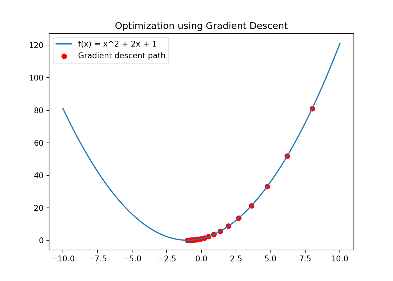

plt.show()

3.4.4.2 2. Numerical Analysis

Numerical methods, such as numerical integration and differentiation, rely on the continuity of functions to provide accurate approximations. Discontinuous functions can lead to large errors or even make the numerical methods inapplicable.

Example: Numerical Integration

Numerical integration methods, like the trapezoidal rule, approximate the area under a curve. Continuity ensures that these approximations are accurate.

from scipy.integrate import quad

def f(x):
    return np.sin(x)

result, error = quad(f, 0, np.pi)
print(f"Numerical integration result: {result}")

## Numerical integration result: 2.0

3.4.4.3 3. Machine Learning

In machine learning, continuous functions are used to model data and make predictions. Activation functions in neural networks, such as the sigmoid and ReLU functions, need to be continuous to ensure smooth gradients during backpropagation, enabling the network to learn effectively.

Example: Activation Functions in Neural Networks

Activation functions introduce non-linearity into neural networks, allowing them to learn complex patterns. Continuous activation functions ensure that the gradients are well-behaved during training.

import numpy as np
import matplotlib.pyplot as plt

def sigmoid(x):
    return 1 / (1 + np.exp(-x))

def relu(x):
    return np.maximum(0, x)

x = np.linspace(-10, 10, 100)
y_sigmoid = sigmoid(x)
y_relu = relu(x)

plt.plot(x, y_sigmoid, label='Sigmoid')

## [<matplotlib.lines.Line2D object at 0x0000029F56FD8AC0>]

plt.plot(x, y_relu, label='ReLU')

## [<matplotlib.lines.Line2D object at 0x0000029F56FE3400>]

plt.legend()

## <matplotlib.legend.Legend object at 0x0000029F56FE3EB0>

plt.title('Continuous Activation Functions')

## Text(0.5, 1.0, 'Continuous Activation Functions')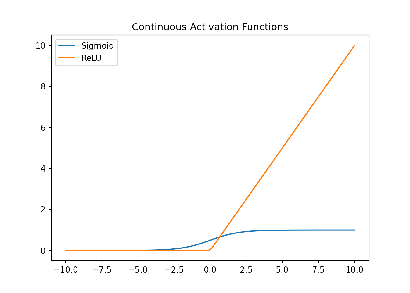

plt.show()

#### 4. Computer Graphics

In computer graphics, continuity is essential for rendering smooth curves and surfaces. Techniques like Bézier curves and B-splines rely on continuous functions to create visually appealing graphics.

Example: Bezier Curves

Bezier curves are used in vector graphics and animation to model smooth curves. The continuity of the curve ensures smooth transitions between points.

import numpy as np
import matplotlib.pyplot as plt

def bezier(t, P0, P1, P2, P3):
    return (1 - t)**3 * P0 + 3 * (1 - t)**2 * t * P1 + 3 * (1 - t) * t**2 * P2 + t**3 * P3

t = np.linspace(0, 1, 100)
P0, P1, P2, P3 = np.array([0, 0]), np.array([1, 2]), np.array([3, 3]), np.array([4, 0])
curve = bezier(t, P0, P1, P2, P3)

plt.plot(curve[:, 0], curve[:, 1], label='Bezier Curve')
plt.scatter([P0[0], P1[0], P2[0], P3[0]], color='red')
plt.title('Bezier Curve in Computer Graphics')
plt.legend()
plt.show()

3.4.4.4 Practical Example of Continuity in Game Design: Smooth Character Movement with Animation

Problem Statement:

In game design, ensuring smooth and natural character movement is essential for a good player experience. Discontinuous or jerky movements can disrupt gameplay and reduce immersion. We will model and animate a character’s movement in a 2D platformer game to ensure smooth transitions.

Mathematical Modelling:

We’ll model the character’s position \(x(t)\) and \(y(t)\) over time \(t\). The movement is influenced by constant velocities in both horizontal and vertical directions.

The equations for position are: \[ x(t) = x_0 + v_x \cdot t \] \[ y(t) = y_0 + v_y \cdot t \]

where: - \(x_0\) and \(y_0\) are the initial positions. - \(v_x\) and \(v_y\) are the constant velocities in the x and y directions, respectively.

Solution:

1. Model the Movement: Update the position continuously based on the time elapsed.

2. Animate the Movement: Create an animation to visualize the smooth movement of the character.

Python Animation Code:

We will use the matplotlib library to create an animation of the character’s movement.

import numpy as np
import matplotlib.pyplot as plt
import matplotlib.animation as animation

# Constants
v_x = 5  # Velocity in x direction
v_y = 3  # Velocity in y direction
x_0 = 0   # Initial x position
y_0 = 0   # Initial y position

# Time array
t = np.linspace(0, 10, 500)  # Time from 0 to 10 seconds

# Position functions
x_t = x_0 + v_x * t
y_t = y_0 + v_y * t

# Create a figure and axis for plotting
fig, ax = plt.subplots()
ax.set_xlim(0, max(x_t) + 10)
ax.set_ylim(min(y_t) - 10, max(y_t) + 10)
line, = ax.plot([], [], 'bo', markersize=10)  # Character represented as a blue dot
trail, = ax.plot([], [], 'b-', alpha=0.5)  # Character's path

def init():
    line.set_data([], [])
    trail.set_data([], [])
    return line, trail

def update(frame):
    line.set_data(x_t[frame], y_t[frame])
    trail.set_data(x_t[:frame+1], y_t[:frame+1])
    return line, trail

# Create animation
ani = animation.FuncAnimation(fig, update, frames=len(t), init_func=init, blit=True, interval=20)

plt.xlabel('X Position')
plt.ylabel('Y Position')
plt.title('Smooth Character Movement in 2D Space')
plt.grid(True)
plt.show()

3.4.4.5 Practical Example of Continuity in Game Design: Smooth Character Movement with Animation

Problem Statement:

In game design, ensuring smooth and natural character movement is essential for a good player experience. Discontinuous or jerky movements can disrupt gameplay and reduce immersion. We will model and animate a character’s movement in a 2D platformer game to ensure smooth transitions.

Mathematical Modelling:

We’ll model the character’s position \(x(t)\) and \(y(t)\) over time \(t\). The movement is influenced by constant velocities in both horizontal and vertical directions.

The equations for position are: \[ x(t) = x_0 + v_x \cdot t \] \[ y(t) = y_0 + v_y \cdot t \]

where: - \(x_0\) and \(y_0\) are the initial positions. - \(v_x\) and \(v_y\) are the constant velocities in the x and y directions, respectively.

Solution:

1. Model the Movement: Update the position continuously based on the time elapsed.

2. Animate the Movement: Create an animation to visualize the smooth movement of the character.

Python Animation Code:

We will use the matplotlib library to create an animation of the character’s movement.

import numpy as np
import matplotlib.pyplot as plt
import matplotlib.animation as animation

# Constants
v_x = 5  # Velocity in x direction
v_y = 3  # Velocity in y direction
x_0 = 0   # Initial x position
y_0 = 0   # Initial y position

# Time array
t = np.linspace(0, 10, 500)  # Time from 0 to 10 seconds

# Position functions
x_t = x_0 + v_x * t
y_t = y_0 + v_y * t

# Create a figure and axis for plotting
fig, ax = plt.subplots()
ax.set_xlim(0, max(x_t) + 10)
ax.set_ylim(min(y_t) - 10, max(y_t) + 10)
line, = ax.plot([], [], 'bo', markersize=10)  # Character represented as a blue dot
trail, = ax.plot([], [], 'b-', alpha=0.5)  # Character's path

def init():
    line.set_data([], [])
    trail.set_data([], [])
    return line, trail

def update(frame):
    line.set_data(x_t[frame], y_t[frame])
    trail.set_data(x_t[:frame+1], y_t[:frame+1])
    return line, trail

# Create animation
ani = animation.FuncAnimation(fig, update, frames=len(t), init_func=init, blit=True, interval=20)

plt.xlabel('X Position')
plt.ylabel('Y Position')
plt.title('Smooth Character Movement in 2D Space')
plt.grid(True)
plt.show()

3.5 Rate of Change

Building on our understanding of limits and continuity, we can now explore the concept of the rate of change, which is crucial for analyzing and optimizing various computational processes in computer science and engineering.

3.5.1 Definition of Rate of Change

The rate of change of a function \(f(x)\) at a particular point \(x\) describes how \(f(x)\) varies as \(x\) changes. Mathematically, it is defined using the concept of a derivative. For a function \(f(x)\), the derivative at a point \(a\) is given by:

\[ f'(a) = \lim_{h \to 0} \frac{f(a+h) - f(a)}{h} \]

This formula represents the instantaneous rate of change of \(f\) with respect to \(x\) at the point \(x = a\).

3.5.2 Practical Applications in Computer Science

1. Algorithm Analysis: The rate of change helps in determining the time complexity of algorithms. For instance, analyzing how the running time of an algorithm increases as the input size grows can be understood through derivatives.
2. Network Traffic Management: Understanding the rate of data flow in networks can help in optimizing bandwidth usage and avoiding congestion.
3. Machine Learning: In gradient-based optimization methods, such as gradient descent, the derivative (or gradient) is used to update model parameters to minimize the loss function.
4. Signal Processing: The rate of change of signals can be analyzed to filter noise and improve signal quality.
5. Graphics and Animation: Smooth rendering of graphics and animations often involves understanding the rate of change of various parameters to create realistic movements and transitions.

3.5.2.1 Visualizing Rate of Change with Python

To make this concept more tangible, let’s use Python and the turtle library to visualize the rate of change for the function \(y = x^2\). We’ll draw the function and dynamically show the tangent line at any point you click, representing the instantaneous rate of change at that point.

Python Code for Visualization: You can visualize the rate of change of \(f(x)\) as tangent at \(x\) using the following Python code (preferably in vscode or pycharm IDEs).

import turtle

# Setup the screen
screen = turtle.Screen()
screen.bgcolor("white")
screen.setup(width=600, height=600)  # Set window size
screen.setworldcoordinates(-6, -1, 6, 36)  # Set coordinate system to match the function range

# Create a turtle object for drawing the function
pen = turtle.Turtle()
pen.speed(0)  # Fastest drawing speed

# Function to draw the quadratic function y = x^2
def draw_function():
    pen.penup()
    pen.goto(-6, 36)  # Move to the starting point
    pen.pendown()
    for x in range(-300, 301):
        x_scaled = x / 50
        y = x_scaled ** 2  # Quadratic function
        pen.goto(x_scaled, y)
    pen.penup()

# Function to draw the tangent line at a given point
def draw_tangent(x, y):
    h = 0.01  # A small increment
    f_a = (x) ** 2  # Function value at x
    f_a_h = (x + h) ** 2  # Function value at x + h
    slope = (f_a_h - f_a) / h  # Derivative (slope) using the limit definition
    
    # Create a new turtle for drawing the tangent
    tangent_pen = turtle.Turtle()
    tangent_pen.speed(0)
    tangent_pen.color("red")
    
    tangent_pen.penup()
    tangent_pen.goto(x, y)
    tangent_pen.pendown()
    
    # Draw the tangent line within the visible range
    tangent_pen.goto(x + 1, y + slope * 1)
    tangent_pen.penup()
    tangent_pen.goto(x, y)
    tangent_pen.pendown()
    tangent_pen.goto(x - 1, y - slope * 1)
    
    tangent_pen.hideturtle()

# Function to handle mouse click events
def on_click(x, y):
    # Adjust y-coordinate to the quadratic function
    y_adjusted = x ** 2
    draw_tangent(x, y_adjusted)

# Draw the function
draw_function()

# Set the mouse click event handler
screen.onclick(on_click)

# Hide the main pen and display the window
pen.hideturtle()
turtle.done()

3.5.2.2 Example 1: Shading a Sphere in Computer Graphics**

In computer graphics, shading techniques are used to create realistic visuals by simulating how light interacts with surfaces. The rate of change is crucial in determining how light intensity varies across the surface of an object, such as a sphere.

Mathematical Model

To shade a sphere realistically, we use the concept of the surface normal and the dot product between the light direction and the normal vector. The intensity of light at a point on the surface is influenced by these factors.

1. Surface Normal Vector: For a sphere centered at the origin with radius \(R\), the surface normal at a point \((x, y, z)\) on the sphere is:

   \[ \mathbf{n} = \frac{(x, y, z)}{R} \]

2. Light Direction Vector: Suppose the light source is located at \((L_x, L_y, L_z)\). The light direction vector at a point on the sphere is:

   \[ \mathbf{L} = (L_x - x, L_y - y, L_z - z) \]

3. Dot Product: The dot product of the surface normal and the light direction vectors is used to compute the intensity of light at that point:

   \[ I = \mathbf{n} \cdot \mathbf{L} \]

   where \(\cdot\) denotes the dot product.

4. Shading Intensity: To ensure the shading intensity is within a valid range, it is often clamped to a minimum value of 0:

   \[ I = \max(0, \mathbf{n} \cdot \mathbf{L}) \]

Python Code for Visualizing Shading on a Sphere

Below is an example code snippet using Python with matplotlib to visualize the shading of a sphere:

import numpy as np
import matplotlib.pyplot as plt
from mpl_toolkits.mplot3d import Axes3D

# Parameters
R = 1  # Radius of the sphere
L = np.array([1, 1, 1])  # Light source position

# Generate spherical coordinates
phi, theta = np.mgrid[0:2*np.pi:100j, 0:np.pi:50j]
x = R * np.sin(theta) * np.cos(phi)
y = R * np.sin(theta) * np.sin(phi)
z = R * np.cos(theta)

# Compute normals
normals = np.stack([x, y, z], axis=-1) / R

# Compute light direction vectors
light_directions = np.stack([L[0] - x, L[1] - y, L[2] - z], axis=-1)

# Compute dot products (shading intensity)
intensities = np.maximum(0, np.sum(normals * light_directions, axis=-1))

# Plotting the sphere with shading
fig = plt.figure()
ax = fig.add_subplot(111, projection='3d')
ax.plot_surface(x, y, z, facecolors=plt.cm.gray(intensities), rstride=5, cstride=5, antialiased=True)

## <mpl_toolkits.mplot3d.art3d.Poly3DCollection object at 0x0000029F571CAD90>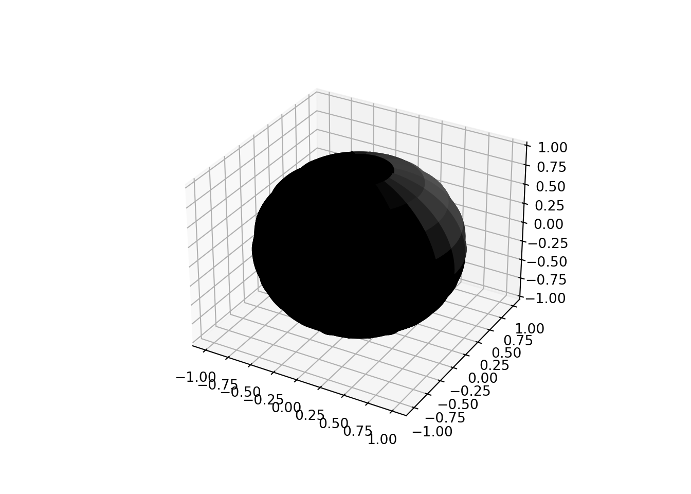

plt.show()

Explanation of terms and notations used:

1. Surface Normal: The surface normal at any point on the sphere is a unit vector pointing outward, which is essential for calculating how light interacts with the surface.

2. Light Direction: The vector from the point on the sphere to the light source determines the angle at which light hits the surface.

3. Dot Product: The dot product between the normal and light direction vectors gives the shading intensity, which is used to color the surface.

3.5.2.3 Example 2: Animating a Bouncing Ball

In animation, the rate of change is crucial for simulating realistic motion. For example, animating a bouncing ball involves understanding how position, velocity, and acceleration change over time.

Mathematical Model:

To simulate the bouncing ball, we use the following kinematic equations:

1. Position as a Function of Time: \(h(t)\)

   • The height \(h(t)\) of the ball at time \(t\) is updated based on its velocity and acceleration.

2. Velocity as a Function of Time: \(v(t)\)

   • The velocity \(v(t)\) changes due to gravity, which is a constant acceleration \(g\).

   The equations are:

   \[ h(t + \Delta t) = h(t) + v(t) \Delta t \]

   \[ v(t + \Delta t) = v(t) - g \Delta t \]

   where:

   • \(g\) is the acceleration due to gravity (\(\approx 9.81 \, \text{m/s}^2\)).
   • \(\Delta t\) is the time step.

3. Handling Bounces: When the ball hits the ground, its velocity is reversed and reduced by a coefficient of restitution \(e\):

   \[ v(t + \Delta t) = -e \cdot v(t) \]

   where \(e\) represents the bounciness of the ball.

Python Code for Visualizing a Bouncing Ball Animation:

Below is an example code snippet using Python with matplotlib to visualize the bouncing ball:

import numpy as np
import matplotlib.pyplot as plt
import matplotlib.animation as animation

# Parameters
g = 9.81  # Acceleration due to gravity (m/s^2)
v_init = 15  # Initial velocity (m/s)
h_init = 0  # Initial height (m)
dt = 0.01  # Time step (s)
e = 0.8  # Coefficient of restitution (bounciness)

# Initial conditions
t = 0  # Initial time
h = h_init  # Initial height
v = v_init  # Initial velocity

# Lists to store the position and time values
positions = []
times = []

# Function to update the position and velocity
def update_position_velocity(h, v, dt):
    h_new = h + v * dt
    v_new = v - g * dt
    return h_new, v_new

# Simulation loop
while t < 5:
    positions.append(h)
    times.append(t)
    h, v = update_position_velocity(h, v, dt)
    if h <= 0:
        h = 0
        v = -v * e
    t += dt

# Create the animation
fig, ax = plt.subplots()
ax.set_xlim(0, 5)
ax.set_ylim(0, max(positions) + 1)
line, = ax.plot([], [], 'o', markersize=10)

def init():
    line.set_data([], [])
    return line,

def animate(i):
    line.set_data(times[i], positions[i])
    return line,

ani = animation.FuncAnimation(fig, animate, frames=len(times), init_func=init, blit=True, interval=dt*1000)
plt.show()

Explanation of terms and constructs used:

1. Position and Velocity: The height \(h\) and velocity \(v\) of the ball are updated iteratively. The position changes based on the current velocity, and the velocity changes based on acceleration due to gravity.

2. Bounce Dynamics: When the ball reaches the ground (height \(\leq 0\)), the velocity is reversed and scaled by the coefficient of restitution, which simulates the bounce effect.

3. Rate of Change: The rate of change of position (velocity) and the rate of change of velocity (acceleration) are key to simulating realistic motion.

3.5.3 Takeaway

The rate of change is a fundamental concept in calculus that finds extensive applications in computer science. By understanding and visualizing how functions change at specific points, computer science students can gain deeper insights into various computational processes and enhance their problem-solving skills.

3.6 Transition from Rate of Change to First Derivative

In our previous discussions, we explored the concept of rate of change in various contexts. We used this idea to understand how quantities such as shading intensity in graphics or position in animation change over time or space. This concept can be formally connected to the mathematical idea of derivatives.

3.6.1 From Rate of Change to Derivatives

The rate of change describes how one quantity changes relative to another. When we talk about the rate of change over an interval, we are referring to the average rate of change. However, to analyze how a function behaves at an exact point, we need to consider the instantaneous rate of change. This is where derivatives come into play.

3.6.2 Instantaneous Rate of Change

While the average rate of change over an interval can be insightful, the derivative provides a precise measure of how a function changes at a specific point. The derivative of a function at a point is essentially the limit of the average rate of change as the interval approaches zero. This captures the instantaneous rate of change.

3.6.3 Definition of the Derivative

The derivative of a function provides a new function that describes the rate of change of the original function at any given point. This new function, known as the derivative function, gives us important insights into the behavior of the original function, including its slope at any point and how that slope changes over different regions.

Concept: Given a function \(f(x)\), its derivative \(f'(x)\) is a function that gives the slope of the tangent to the graph of \(f(x)\) at any point \(x\). The derivative function \(f'(x)\) itself can be analyzed to understand how the rate of change of \(f(x)\) varies:

• Rate of Change: The derivative function \(f'(x)\) tells us how quickly \(f(x)\) is changing at each point \(x\).
• Slope of Tangent: At any point on the curve of \(f(x)\), the value of \(f'(x)\) represents the slope of the tangent line at that point.

Formally, the derivative of a function \(f(x)\) at a point \(x\) is defined as:

\[ f'(x) = \lim_{h \to 0} \frac{f(x + h) - f(x)}{h} \]

This definition states that the derivative \(f'(x)\) is the limit of the average rate of change of the function as the interval \(h\) approaches zero. This limit must be instantaneous to accurately reflect how the function is changing at exactly \(x\).

Key Points o remember:

1. Rate of Change: Refers to how a function changes over an interval.
2. Instantaneous Rate of Change: Requires the interval to be infinitesimally small, capturing how the function changes precisely at a point.
3. Derivative: The limit of the average rate of change as the interval approaches zero, providing a precise measure of the instantaneous rate of change.

Example:

Consider a simple function \(f(x) = x^2\). The rate of change between two points \(x\) and \(x + h\) is:

\[ \frac{f(x + h) - f(x)}{h} = \frac{(x + h)^2 - x^2}{h} = \frac{2xh + h^2}{h} = 2x + h \]

As \(h\) approaches zero, the rate of change approaches \(2x\), which is the derivative of \(f(x)\):

\[ f'(x) = \lim_{h \to 0} \left(2x + h\right) = 2x \]

Here, \(2x\) represents the instantaneous rate of change of the function \(f(x) = x^2\) at any point \(x\).

This means the derivative function \(f'(x) = 2x\) tells us that the slope of the tangent line to the curve \(f(x) = x^2\) at any point \(x\) is \(2x\). For instance: - At \(x = 1\), the slope of the tangent line is \(2 \times 1 = 2\). - At \(x = -2\), the slope of the tangent line is \(2 \times (-2) = -4\).

Visualization

To visualize the derivative as a function, we can plot the original function along with its derivative:

import numpy as np
import matplotlib.pyplot as plt

# Define the function and its derivative
def f(x):
    return x**2

def f_prime(x):
    return 2*x

# Define the x values
x = np.linspace(-3, 3, 400)
y = f(x)
y_prime = f_prime(x)

# Create a figure with subplots
plt.figure(figsize=(12, 8))

## <Figure size 1200x800 with 0 Axes>

# Plot the function
plt.plot(x, y, label='$f(x) = x^2$', color='blue')

## [<matplotlib.lines.Line2D object at 0x0000029F57409D60>]

# Plot the derivative
plt.plot(x, y_prime, label="$f'(x) = 2x$", color='green', linestyle='--')

## [<matplotlib.lines.Line2D object at 0x0000029F57414370>]

# Annotate the plot
plt.title('Function and Its Derivative')

## Text(0.5, 1.0, 'Function and Its Derivative')

plt.xlabel('x')

## Text(0.5, 0, 'x')

plt.ylabel('y')

## Text(0, 0.5, 'y')

plt.axhline(0, color='black',linewidth=0.5)

## <matplotlib.lines.Line2D object at 0x0000029F574189D0>

plt.axvline(0, color='black',linewidth=0.5)

## <matplotlib.lines.Line2D object at 0x0000029F57420D30>

plt.grid(True)
plt.legend()

## <matplotlib.legend.Legend object at 0x0000029F574207F0>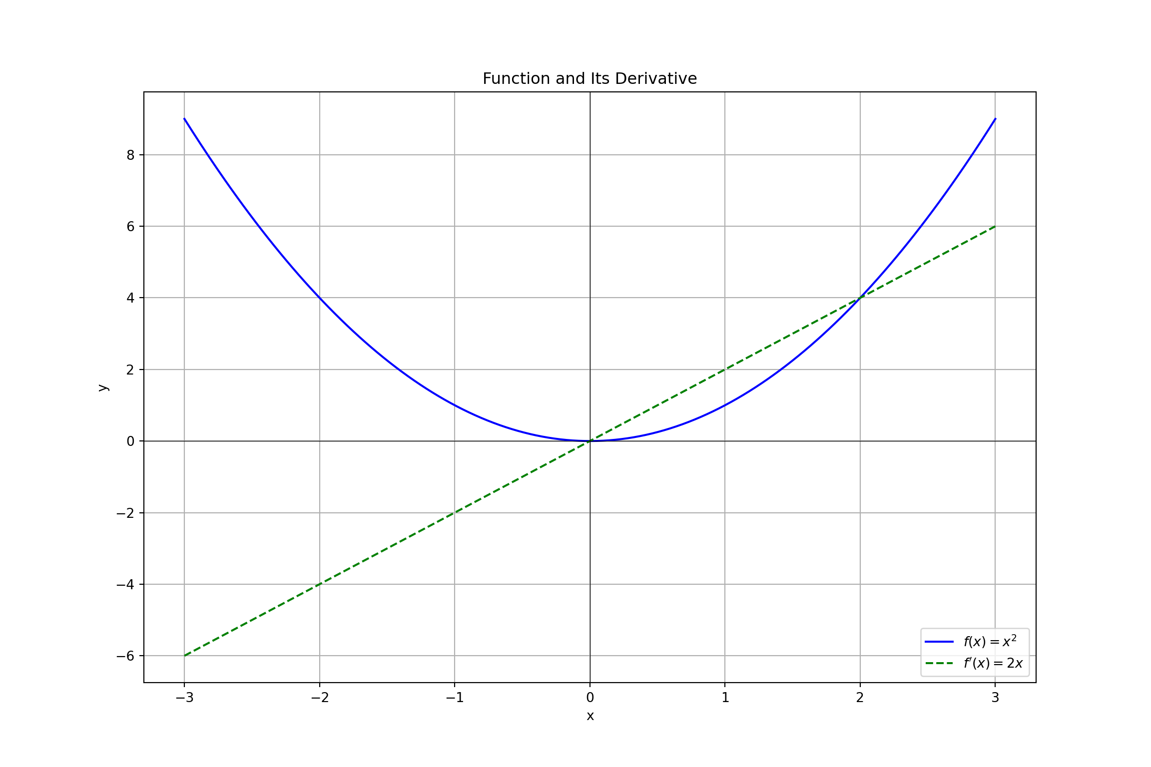

plt.show()

By transitioning from the average rate of change to the instantaneous rate of change, we use the concept of the derivative. The derivative provides a precise measure of how a function behaves at a particular point, capturing the essence of instantaneous change. This concept is fundamental in various applications, from optimization in machine learning to dynamic simulations in computer graphics.

3.6.4 Chain Rule in Differentiation

The Chain Rule is a fundamental technique in calculus used to differentiate composite functions. In practical terms, the Chain Rule helps us determine how a function changes when it is composed of other functions. This is particularly useful in computer science and engineering when dealing with complex functions or systems where one function is nested within another.

Concept:

The Chain Rule states that if you have a composite function \(g(f(x))\), where: - \(f(x)\) is an inner function - \(g(u)\) is an outer function, where \(u = f(x)\)

then the derivative of the composite function \(g(f(x))\) with respect to \(x\) is given by:

\[ \frac{d}{dx} [g(f(x))] = g'(f(x)) \cdot f'(x) \]

Note: In simpler terms, the derivative of the composite function is the derivative of the outer function evaluated at the inner function multiplied by the derivative of the inner function.

Practical Example:

Consider a scenario in computer graphics where you need to compute the rate of change of color intensity on a surface, which depends on a parameter such as light intensity. Let’s break it down into a practical example:

• Inner Function \(f(x)\): Represents the light intensity as a function of some parameter \(x\).
• Outer Function \(g(u)\): Represents the color intensity as a function of light intensity \(u\), where \(u = f(x)\).

Suppose: - The inner function \(f(x) = x^2\) represents how light intensity changes with parameter \(x\). - The outer function \(g(u) = \sqrt{u}\) represents how color intensity changes with light intensity \(u\).

To find the rate of change of color intensity with respect to \(x\), use the Chain Rule:

1. Differentiate the inner function \(f(x)\): \[ f'(x) = 2x \]

2. Differentiate the outer function \(g(u)\): \[ g'(u) = \frac{1}{2\sqrt{u}} \]

3. Apply the Chain Rule: \[ \frac{d}{dx} [g(f(x))] = g'(f(x)) \cdot f'(x) \] Substituting \(f(x) = x^2\) into \(g'(u)\): \[ \frac{d}{dx} [\sqrt{x^2}] = \frac{1}{2\sqrt{x^2}} \cdot 2x = \frac{x}{\sqrt{x^2}} \] Simplifying, we get: \[ \frac{d}{dx} [\sqrt{x^2}] = \text{sgn}(x) \] where \(\text{sgn}(x)\) is the sign function that indicates the sign of \(x\).

Practical Visualization

In programming or simulations, applying the Chain Rule often involves writing functions that call other functions. Here’s an example in Python:

import numpy as np
import matplotlib.pyplot as plt

# Define the inner function and its derivative
def f(x):
    return x**2

def f_prime(x):
    return 2*x

# Define the outer function and its derivative
def g(u):
    return np.sqrt(u)

def g_prime(u):
    return 1 / (2 * np.sqrt(u))

# Define the composite function and its derivative
def composite_function(x):
    return g(f(x))

def composite_derivative(x):
    return g_prime(f(x)) * f_prime(x)

# Define the x values
x = np.linspace(-5, 5, 400)
y = composite_function(x)
y_prime = composite_derivative(x)

# Create the plot
plt.figure(figsize=(10, 6))

## <Figure size 1000x600 with 0 Axes>

# Plot the composite function
plt.plot(x, y, label='$g(f(x)) = \sqrt{x^2}$', color='blue')

## [<matplotlib.lines.Line2D object at 0x0000029F56713E20>]

# Plot the derivative of the composite function
plt.plot(x, y_prime, label="Derivative: $\text{sgn}(x)$", color='green', linestyle='--')

## [<matplotlib.lines.Line2D object at 0x0000029F56758FA0>]

# Annotate the plot
plt.title('Composite Function and Its Derivative')

## Text(0.5, 1.0, 'Composite Function and Its Derivative')

plt.xlabel('x')

## Text(0.5, 0, 'x')

plt.ylabel('y')

## Text(0, 0.5, 'y')

plt.axhline(0, color='black', linewidth=0.5)

## <matplotlib.lines.Line2D object at 0x0000029F56A45940>

plt.axvline(0, color='black', linewidth=0.5)

## <matplotlib.lines.Line2D object at 0x0000029F56DAB370>

plt.grid(True)
plt.legend()

## <matplotlib.legend.Legend object at 0x0000029F56A45E80>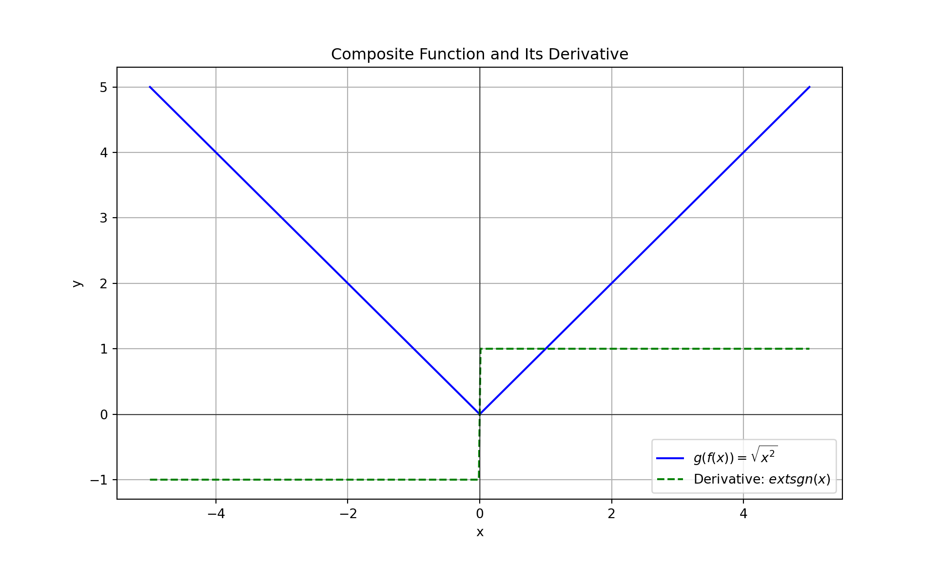

plt.show()

To find derivative of functions, we need standard rules of differentiation. Laws of differentiation is shown in following table.

3.6.5 Basic Rules in Differentiation

Rule	Formula	Description
Constant Rule	\(\frac{d}{dx}[c] = 0\)	The derivative of a constant \(c\) is zero.
Power Rule	\(\frac{d}{dx}[x^n] = nx^{n-1}\)	For \(n\) a real number, the derivative of \(x^n\) is \(nx^{n-1}\).
Constant Multiple Rule	\(\frac{d}{dx}[cf(x)] = c \cdot f'(x)\)	The derivative of \(cf(x)\) is \(c\) times the derivative of \(f(x)\).
Sum Rule	\(\frac{d}{dx}[f(x) + g(x)] = f'(x) + g'(x)\)	The derivative of a sum is the sum of the derivatives.
Difference Rule	\(\frac{d}{dx}[f(x) - g(x)] = f'(x) - g'(x)\)	The derivative of a difference is the difference of the derivatives.
Product Rule	\(\frac{d}{dx}[f(x) \cdot g(x)] = f'(x) \cdot g(x) + f(x) \cdot g'(x)\)	The derivative of a product is given by: \(f'(x) \cdot g(x) + f(x) \cdot g'(x)\).
Quotient Rule	\(\frac{d}{dx}\left[\frac{f(x)}{g(x)}\right] = \frac{f'(x) \cdot g(x) - f(x) \cdot g'(x)}{[g(x)]^2}\)	The derivative of a quotient is \(\frac{f'(x) \cdot g(x) - f(x) \cdot g'(x)}{[g(x)]^2}\).
Chain Rule	\(\frac{d}{dx}[f(g(x))] = f'(g(x)) \cdot g'(x)\)	The derivative of a composite function is the derivative of the outer function evaluated at the inner function, multiplied by the derivative of the inner function.
Exponential Rule	\(\frac{d}{dx}[e^x] = e^x\)	The derivative of \(e^x\) is \(e^x\).
Logarithmic Rule	\(\frac{d}{dx}[\ln(x)] = \frac{1}{x}\)	The derivative of \(\ln(x)\) is \(\frac{1}{x}\).
Trigonometric Functions	\(\frac{d}{dx}[\sin(x)] = \cos(x)\) \(\frac{d}{dx}[\cos(x)] = -\sin(x)\) \(\frac{d}{dx}[\tan(x)] = \sec^2(x)\)	Derivatives of common trigonometric functions: \(\sin(x)\), \(\cos(x)\), and \(\tan(x)\).

3.6.5.1 Practice Problems for Basic Differentiation Rules

Constant Rule

Problems:

1. Find the derivative of \(f(x) = 7\).
2. Find the derivative of \(f(x) = -3\).
3. Find the derivative of \(f(x) = \pi\).
4. Find the derivative of \(f(x) = 0\).
5. Find the derivative of \(f(x) = \sqrt{2}\).

Solutions:

1. Solution: \(\frac{d}{dx}[7] = 0\)
2. Solution: \(\frac{d}{dx}[-3] = 0\)
3. Solution: \(\frac{d}{dx}[\pi] = 0\)
4. Solution: \(\frac{d}{dx}[0] = 0\)
5. Solution: \(\frac{d}{dx}[\sqrt{2}] = 0\)

---

Power Rule

Problems:

1. Find the derivative of \(f(x) = x^5\).
2. Find the derivative of \(f(x) = x^{-2}\).
3. Find the derivative of \(f(x) = x^{1/2}\).
4. Find the derivative of \(f(x) = 4x^3\).
5. Find the derivative of \(f(x) = \frac{1}{x^4}\).

Solutions:

1. Solution: \(\frac{d}{dx}[x^5] = 5x^4\)
2. Solution: \(\frac{d}{dx}[x^{-2}] = -2x^{-3}\)
3. Solution: \(\frac{d}{dx}[x^{1/2}] = \frac{1}{2}x^{-1/2}\)
4. Solution: \(\frac{d}{dx}[4x^3] = 12x^2\)
5. Solution: \(\frac{d}{dx}\left[\frac{1}{x^4}\right] = -4x^{-5}\)

---

Constant Multiple Rule

Problems:

1. Find the derivative of \(f(x) = 3 \cdot x^4\).
2. Find the derivative of \(f(x) = -7 \cdot x^2\).
3. Find the derivative of \(f(x) = 5 \cdot x^{-1}\).
4. Find the derivative of \(f(x) = \frac{2}{3} \cdot x^3\).
5. Find the derivative of \(f(x) = 4 \cdot \sqrt{x}\).

Solutions:

1. Solution: \(\frac{d}{dx}[3x^4] = 12x^3\)
2. Solution: \(\frac{d}{dx}[-7x^2] = -14x\)
3. Solution: \(\frac{d}{dx}[5x^{-1}] = -5x^{-2}\)
4. Solution: \(\frac{d}{dx}\left[\frac{2}{3}x^3\right] = 2x^2\)
5. Solution: \(\frac{d}{dx}[4\sqrt{x}] = 2x^{-1/2}\)

---

Sum Rule

Problems:

1. Find the derivative of \(f(x) = x^3 + 2x^2\).
2. Find the derivative of \(f(x) = 4x^2 - x + 5\).
3. Find the derivative of \(f(x) = \sin(x) + \cos(x)\).
4. Find the derivative of \(f(x) = x^{-1} + e^x\).
5. Find the derivative of \(f(x) = 3x^4 + 2x^3 - x\).

Solutions:

1. Solution: \(\frac{d}{dx}[x^3 + 2x^2] = 3x^2 + 4x\)
2. Solution: \(\frac{d}{dx}[4x^2 - x + 5] = 8x - 1\)
3. Solution: \(\frac{d}{dx}[\sin(x) + \cos(x)] = \cos(x) - \sin(x)\)
4. Solution: \(\frac{d}{dx}\left[x^{-1} + e^x\right] = -x^{-2} + e^x\)
5. Solution: \(\frac{d}{dx}[3x^4 + 2x^3 - x] = 12x^3 + 6x^2 - 1\)

---

Difference Rule

Problems:

1. Find the derivative of \(f(x) = x^3 - 3x^2\).
2. Find the derivative of \(f(x) = e^x - \ln(x)\).
3. Find the derivative of \(f(x) = \tan(x) - \sin(x)\).
4. Find the derivative of \(f(x) = \frac{1}{x^2} - x\).
5. Find the derivative of \(f(x) = 4x^3 - 2x^2 + x - 5\).

Solutions:

1. Solution: \(\frac{d}{dx}[x^3 - 3x^2] = 3x^2 - 6x\)
2. Solution: \(\frac{d}{dx}[e^x - \ln(x)] = e^x - \frac{1}{x}\)
3. Solution: \(\frac{d}{dx}[\tan(x) - \sin(x)] = \sec^2(x) - \cos(x)\)
4. Solution: \(\frac{d}{dx}\left[\frac{1}{x^2} - x\right] = -\frac{2}{x^3} - 1\)
5. Solution: \(\frac{d}{dx}[4x^3 - 2x^2 + x - 5] = 12x^2 - 4x + 1\)

---

Product Rule

Problems:

1. Find the derivative of \(f(x) = x^2 \cdot \sin(x)\).
2. Find the derivative of \(f(x) = e^x \cdot \cos(x)\).
3. Find the derivative of \(f(x) = x \cdot \ln(x)\).
4. Find the derivative of \(f(x) = x^3 \cdot e^x\).
5. Find the derivative of \(f(x) = \sqrt{x} \cdot \tan(x)\).

Solutions:

1. Solution: \(\frac{d}{dx}[x^2 \sin(x)] = 2x \sin(x) + x^2 \cos(x)\)
2. Solution: \(\frac{d}{dx}[e^x \cos(x)] = e^x \cos(x) - e^x \sin(x)\)
3. Solution: \(\frac{d}{dx}[x \ln(x)] = \ln(x) + 1\)
4. Solution: \(\frac{d}{dx}[x^3 e^x] = x^3 e^x + 3x^2 e^x\)
5. Solution: \(\frac{d}{dx}[\sqrt{x} \cdot \tan(x)] = \frac{1}{2\sqrt{x}} \cdot \tan(x) + \sqrt{x} \cdot \sec^2(x)\)

---

Quotient Rule

Problems:

1. Find the derivative of \(f(x) = \frac{x^2}{\sin(x)}\).
2. Find the derivative of \(f(x) = \frac{e^x}{x}\).
3. Find the derivative of \(f(x) = \frac{\cos(x)}{x^2}\).
4. Find the derivative of \(f(x) = \frac{x \cdot \ln(x)}{x^2 + 1}\).
5. Find the derivative of \(f(x) = \frac{\sqrt{x}}{\tan(x)}\).

Solutions:

1. Solution: \(\frac{d}{dx}\left[\frac{x^2}{\sin(x)}\right] = \frac{2x \sin(x) - x^2 \cos(x)}{\sin^2(x)}\)
2. Solution: \(\frac{d}{dx}\left[\frac{e^x}{x}\right] = \frac{e^x (x - 1)}{x^2}\)
3. Solution: \(\frac{d}{dx}\left[\frac{\cos(x)}{x^2}\right] = \frac{-\sin(x) \cdot x^2 - \cos(x) \cdot 2x}{x^4}\)
4. Solution: \(\frac{d}{dx}\left[\frac{x \ln(x)}{x^2 + 1}\right] = \frac{(x \cdot \frac{1}{x} + \ln(x)) (x^2 + 1) - x \ln(x) \cdot 2x}{(x^2 + 1)^2}\)
5. Solution: \(\frac{d}{dx}\left[\frac{\sqrt{x}}{\tan(x)}\right] = \frac{\frac{1}{2\sqrt{x}} \cdot \tan(x) - \sqrt{x} \cdot \sec^2(x)}{\tan^2(x)}\)

---

Chain Rule

Problems:

1. Find the derivative of \(f(x) = \sin(x^2)\).
2. Find the derivative of \(f(x) = \ln(\cos(x))\).
3. Find the derivative of \(f(x) = e^{\sin(x)}\).
4. Find the derivative of \(f(x) = (3x + 1)^5\).
5. Find the derivative of \(f(x) = \sqrt{\ln(x)}\).

Solutions:

1. Solution: \(\frac{d}{dx}[\sin(x^2)] = \cos(x^2) \cdot 2x\)
2. Solution: \(\frac{d}{dx}[\ln(\cos(x))] = \frac{-\sin(x)}{\cos(x)} = -\tan(x)\)
3. Solution: \(\frac{d}{dx}[e^{\sin(x)}] = e^{\sin(x)} \cdot \cos(x)\)
4. Solution: \(\frac{d}{dx}[(3x + 1)^5] = 5(3x + 1)^4 \cdot 3\)
5. Solution: \(\frac{d}{dx}[\sqrt{\ln(x)}] = \frac{1}{2\sqrt{\ln(x)}} \cdot \frac{1}{x}\)

---

Exponential Rule

Problems:

1. Find the derivative of \(f(x) = e^{3x}\).
2. Find the derivative of \(f(x) = 2e^x\).
3. Find the derivative of \(f(x) = e^{-x}\).
4. Find the derivative of \(f(x) = e^{x^2}\).
5. Find the derivative of \(f(x) = e^{\sin(x)}\).

Solutions:

1. Solution: \(\frac{d}{dx}[e^{3x}] = 3e^{3x}\)
2. Solution: \(\frac{d}{dx}[2e^x] = 2e^x\)
3. Solution: \(\frac{d}{dx}[e^{-x}] = -e^{-x}\)
4. Solution: \(\frac{d}{dx}[e^{x^2}] = 2x e^{x^2}\)
5. Solution: \(\frac{d}{dx}[e^{\sin(x)}] = e^{\sin(x)} \cdot \cos(x)\)

---

Logarithmic Rule

Problems:

1. Find the derivative of \(f(x) = \ln(x^2 + 1)\).
2. Find the derivative of \(f(x) = \ln(3x)\).
3. Find the derivative of \(f(x) = \ln(\sin(x))\).
4. Find the derivative of \(f(x) = \ln(x^3 + x)\).
5. Find the derivative of \(f(x) = \ln(e^x + 1)\).

Solutions:

1. Solution: \(\frac{d}{dx}[\ln(x^2 + 1)] = \frac{2x}{x^2 + 1}\)
2. Solution: \(\frac{d}{dx}[\ln(3x)] = \frac{1}{x}\)
3. Solution: \(\frac{d}{dx}[\ln(\sin(x))] = \cot(x)\)
4. Solution: \(\frac{d}{dx}[\ln(x^3 + x)] = \frac{3x^2 + 1}{x^3 + x}\)
5. Solution: \(\frac{d}{dx}[\ln(e^x + 1)] = \frac{e^x}{e^x + 1}\)

---

3.6.6 Implicit Differentiation

Implicit Differentiation is a technique used to find the derivative of a function when it is not explicitly defined in terms of one variable. Instead, the function is given in an implicit form, where the variables are mixed together in an equation. This method is crucial when dealing with equations where solving for one variable in terms of another is difficult or impossible.

Concept: When a function \(y\) is defined implicitly by an equation involving both \(x\) and \(y\), such as:

\[ F(x, y) = 0 \]

where \(F\) is a function of both \(x\) and \(y\), implicit differentiation allows us to find \(\frac{dy}{dx}\) without explicitly solving for \(y\) as a function of \(x\).

To perform implicit differentiation, follow these steps:

1. Differentiate both sides of the equation with respect to \(x\), treating \(y\) as an implicit function of \(x\).
2. Apply the chain rule when differentiating terms involving \(y\), because \(\frac{dy}{dx}\) is present in those terms.
3. Solve for \(\frac{dy}{dx}\) to find the derivative.

Necessity in Application: Implicit differentiation is particularly useful in several scenarios:

• Complex Relationships: When dealing with curves defined by equations that are difficult to solve for \(y\) explicitly.
• Conic Sections and Ellipses: In engineering and physics problems where the equations of curves are given in implicit form.
• Machine Learning: When optimizing loss functions where constraints are given implicitly.
• Computer Graphics: When modeling curves and surfaces where explicit formulas are hard to derive.

Practical Example:

Consider the circle defined by the equation:

\[ x^2 + y^2 = 1 \]

We want to find the slope of the tangent line to the circle at any point \((x, y)\).

1. Differentiate both sides of the equation with respect to \(x\): \[ \frac{d}{dx}(x^2 + y^2) = \frac{d}{dx}(1) \]

2. Apply the chain rule: \[ 2x + 2y \frac{dy}{dx} = 0 \]

3. Solve for \(\frac{dy}{dx}\): \[ \frac{dy}{dx} = -\frac{x}{y} \]

This result shows how the slope of the tangent to the circle changes depending on the coordinates \((x, y)\).

Python Visualization

Here’s a Python example to visualize the tangent lines to a circle:

import numpy as np
import matplotlib.pyplot as plt

# Define the circle
theta = np.linspace(0, 2 * np.pi, 100)
x_circle = np.cos(theta)
y_circle = np.sin(theta)

# Define points of interest
points = np.array([[-0.5, 0.5], [0.5, -0.5], [0, 1]])

# Create the plot
plt.figure(figsize=(8, 8))

## <Figure size 800x800 with 0 Axes>

# Plot the circle
plt.plot(x_circle, y_circle, label='Circle: $x^2 + y^2 = 1$', color='blue')

## [<matplotlib.lines.Line2D object at 0x0000029F569F9CD0>]

# Plot tangent lines
for point in points:
    x, y = point
    slope = -x / y
    x_tangent = np.linspace(x - 1, x + 1, 10)
    y_tangent = slope * (x_tangent - x) + y
    plt.plot(x_tangent, y_tangent, '--', label=f'Tangent at ({x}, {y})')

## [<matplotlib.lines.Line2D object at 0x0000029F56CC8A90>]
## [<matplotlib.lines.Line2D object at 0x0000029F569E4700>]
## [<matplotlib.lines.Line2D object at 0x0000029F56741BB0>]

# Annotate the plot
plt.scatter(points[:, 0], points[:, 1], color='red')  # Points of interest

## <matplotlib.collections.PathCollection object at 0x0000029F567521F0>

plt.title('Circle and Tangent Lines')

## Text(0.5, 1.0, 'Circle and Tangent Lines')

plt.xlabel('x')

## Text(0.5, 0, 'x')

plt.ylabel('y')

## Text(0, 0.5, 'y')

plt.axhline(0, color='black', linewidth=0.5)

## <matplotlib.lines.Line2D object at 0x0000029F56D65610>

plt.axvline(0, color='black', linewidth=0.5)

## <matplotlib.lines.Line2D object at 0x0000029F56D81EE0>

plt.grid(True)
plt.legend()

## <matplotlib.legend.Legend object at 0x0000029F57219520>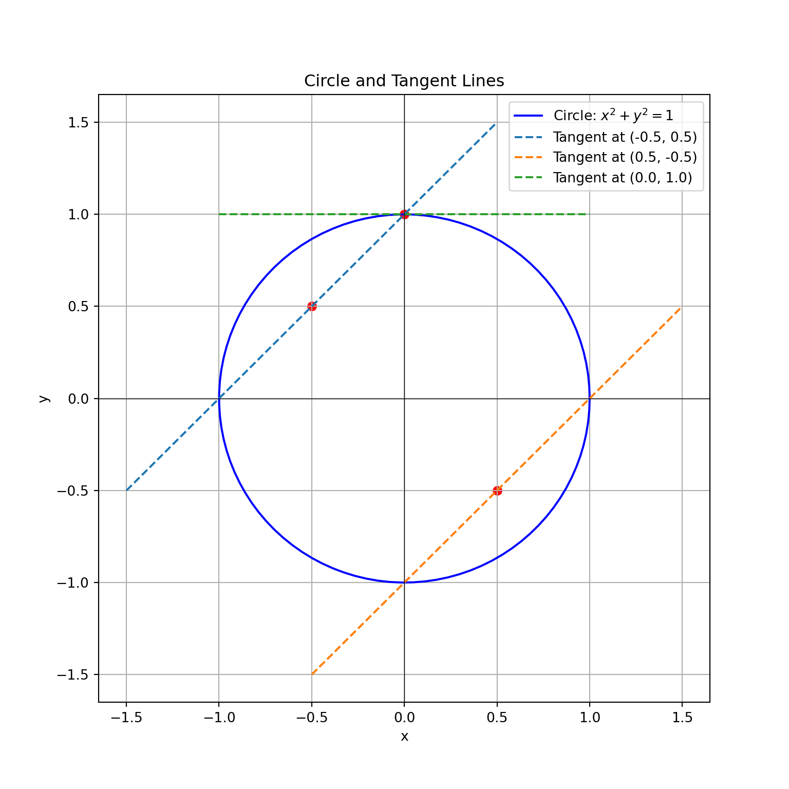

plt.show()

3.6.7 Tangents and Normal Lines

In our previous discussions, we explored the concept of a tangent at a point on a curve. To recap, the tangent line to a function \(f(x)\) at a specific point \(x = x_0\) represents the instantaneous rate of change of the function at that point.

Tangent Line: The tangent line to \(f(x)\) at \(x = x_0\) is the line that just touches the curve at that point, providing the best linear approximation of the function at \(x_0\). The formula for the tangent line is: \[ y - f(x_0) = f'(x_0) (x - x_0) \] where \(f'(x_0)\) is the derivative of \(f(x)\) at \(x_0\), and \((x_0, f(x_0))\) is the point of tangency.

Normal Line: The normal line to \(f(x)\) at \(x = x_0\) is the line perpendicular to the tangent line at that point. It provides insight into the direction in which the curve bends away from the tangent line. The formula for the normal line is: \[ y - f(x_0) = -\frac{1}{f'(x_0)} (x - x_0) \] where \(-\frac{1}{f'(x_0)}\) is the slope of the normal line.

Example: Consider thefFunction \(f(x) = x^2\) at \(x = 2\)

Let’s use the function \(f(x) = x^2\) to find both the tangent and normal lines at \(x = 2\):

1. Find the derivative \(f'(x)\): \[ f'(x) = 2x \]

2. Evaluate the derivative at \(x = 2\): \[ f'(2) = 2 \cdot 2 = 4 \] The slope of the tangent line at \(x = 2\) is \(4\).

3. Write the equation of the tangent line: Using the point-slope form: \[ y - 4 = 4 (x - 2) \] where \(f(2) = 4\). Simplifying: \[ y = 4x - 4 \]

4. Find the slope of the normal line: The slope of the normal line is the negative reciprocal of the tangent line’s slope: \[ \text{slope of normal line} = -\frac{1}{4} \]

5. Write the equation of the normal line: Using the point-slope form: \[ y - 4 = -\frac{1}{4} (x - 2) \] Simplify to: \[ y = -\frac{1}{4}x + \frac{9}{2} \]

Python Visualization

To visualize both the tangent and normal lines for the function \(f(x) = x^2\) at \(x = 2\), use the following Python code:

import numpy as np
import matplotlib.pyplot as plt

# Define the function and its derivative
def f(x):
    return x**2

def f_prime(x):
    return 2*x

# Define the point of interest
x0 = 2
y0 = f(x0)
slope_tangent = f_prime(x0)
slope_normal = -1 / slope_tangent

# Define x values for plotting
x = np.linspace(0, 4, 400)
y = f(x)

# Calculate tangent and normal lines
x_tangent = np.linspace(0, 4, 10)
y_tangent = slope_tangent * (x_tangent - x0) + y0

x_normal = np.linspace(0, 4, 10)
y_normal = slope_normal * (x_normal - x0) + y0

# Create the plot
plt.figure(figsize=(10, 6))

## <Figure size 1000x600 with 0 Axes>

# Plot the function
plt.plot(x, y, label='$f(x) = x^2$', color='blue')

## [<matplotlib.lines.Line2D object at 0x0000029F56FD8790>]

# Plot the tangent line
plt.plot(x_tangent, y_tangent, '--', label='Tangent at $x=2$', color='red')

## [<matplotlib.lines.Line2D object at 0x0000029F569E9BB0>]

# Plot the normal line
plt.plot(x_normal, y_normal, '--', label='Normal at $x=2$', color='green')

## [<matplotlib.lines.Line2D object at 0x0000029F569E9FD0>]

# Annotate the plot
plt.scatter([x0], [y0], color='black')  # Point of tangency

## <matplotlib.collections.PathCollection object at 0x0000029F56A69190>

plt.title('Function, Tangent Line, and Normal Line')

## Text(0.5, 1.0, 'Function, Tangent Line, and Normal Line')

plt.xlabel('x')

## Text(0.5, 0, 'x')

plt.ylabel('y')

## Text(0, 0.5, 'y')

plt.axhline(0, color='black', linewidth=0.5)

## <matplotlib.lines.Line2D object at 0x0000029F56A73D30>

plt.axvline(0, color='black', linewidth=0.5)

## <matplotlib.lines.Line2D object at 0x0000029F56A73040>

plt.grid(True)
plt.legend()

## <matplotlib.legend.Legend object at 0x0000029F569E9820>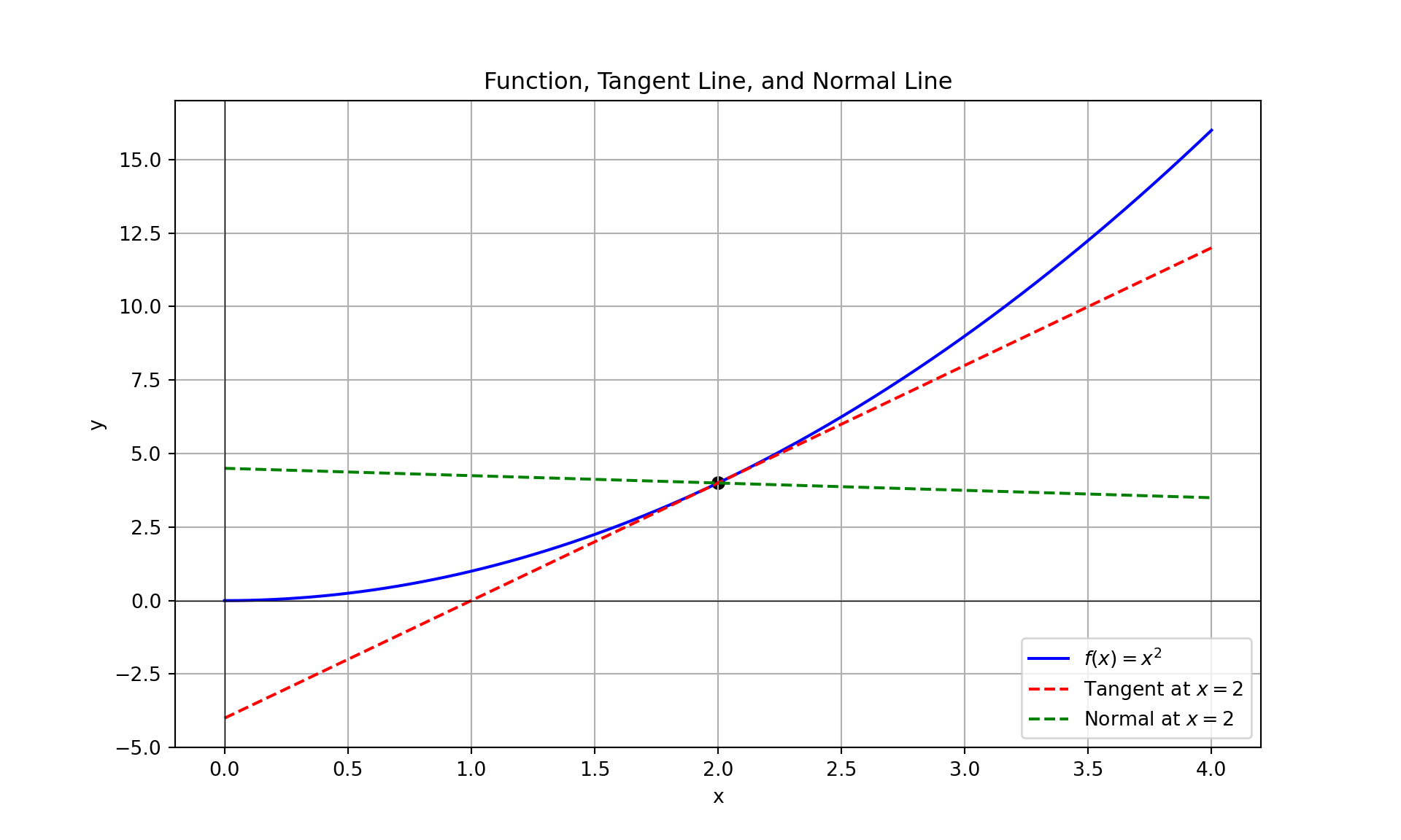

plt.show()

3.6.7.1 Problems on Tangent Line and Normal Line

Problem 1:
Find the equation of the tangent line to the curve \(y = x^2\) at the point \((1, 1)\).

Solution:
1. Find the derivative \(y'\) of the function \(y = x^2\): \[ y' = 2x \] 2. Evaluate the derivative at \(x = 1\): \[ y'(1) = 2(1) = 2 \] 3. Use the point-slope form of the equation of the tangent line: \[ y - y_1 = m(x - x_1) \] \[ y - 1 = 2(x - 1) \] \[ y = 2x - 1 \]

---

Problem 2:
Find the equation of the normal line to the curve \(y = \sqrt{x}\) at the point \((4, 2)\).

Solution:
1. Find the derivative \(y'\) of the function \(y = \sqrt{x}\): \[ y' = \frac{1}{2\sqrt{x}} \] 2. Evaluate the derivative at \(x = 4\): \[ y'(4) = \frac{1}{2\sqrt{4}} = \frac{1}{4} \] 3. The slope of the normal line is the negative reciprocal of the slope of the tangent line: \[ m_{\text{normal}} = -\frac{1}{y'(4)} = -4 \] 4. Use the point-slope form of the equation of the normal line: \[ y - y_1 = m_{\text{normal}}(x - x_1) \] \[ y - 2 = -4(x - 4) \] \[ y = -4x + 18 \]

---

Problem 3:
Find the equation of the tangent line to the curve \(y = e^x\) at the point where \(x = 0\).

Solution:
1. Find the derivative \(y'\) of the function \(y = e^x\): \[ y' = e^x \] 2. Evaluate the derivative at \(x = 0\): \[ y'(0) = e^0 = 1 \] 3. Use the point-slope form of the equation of the tangent line: \[ y - y_1 = m(x - x_1) \] \[ y - 1 = 1(x - 0) \] \[ y = x + 1 \]

---

Problem 4:
Find the equation of the normal line to the curve \(y = \ln(x)\) at the point where \(x = 1\).

Solution:
1. Find the derivative \(y'\) of the function \(y = \ln(x)\): \[ y' = \frac{1}{x} \] 2. Evaluate the derivative at \(x = 1\): \[ y'(1) = 1 \] 3. The slope of the normal line is the negative reciprocal of the slope of the tangent line: \[ m_{\text{normal}} = -\frac{1}{y'(1)} = -1 \] 4. Use the point-slope form of the equation of the normal line: \[ y - y_1 = m_{\text{normal}}(x - x_1) \] \[ y - 0 = -1(x - 1) \] \[ y = -x + 1 \]

---

Problem 5:
Find the equation of the tangent line to the curve \(y = \sin(x)\) at the point where \(x = \frac{\pi}{2}\).

Solution:
1. Find the derivative \(y'\) of the function \(y = \sin(x)\): \[ y' = \cos(x) \] 2. Evaluate the derivative at \(x = \frac{\pi}{2}\): \[ y'(\frac{\pi}{2}) = \cos(\frac{\pi}{2}) = 0 \] 3. Use the point-slope form of the equation of the tangent line: \[ y - y_1 = m(x - x_1) \] \[ y - 1 = 0(x - \frac{\pi}{2}) \] \[ y = 1 \]

---

Problem 6:
Find the equation of the normal line to the curve \(y = \cos(x)\) at the point where \(x = \pi\).

Solution:
1. Find the derivative \(y'\) of the function \(y = \cos(x)\): \[ y' = -\sin(x) \] 2. Evaluate the derivative at \(x = \pi\): \[ y'(\pi) = -\sin(\pi) = 0 \] 3. The slope of the normal line is the negative reciprocal of the slope of the tangent line: \[ m_{\text{normal}} \text{ is undefined (as the slope of the tangent is zero)} \] 4. The normal line is vertical at \(x = \pi\), so its equation is: \[ x = \pi \]

---

Problem 7:
Find the equation of the tangent line to the curve \(y = x^3 - 3x + 2\) at the point where \(x = 1\).

Solution:
1. Find the derivative \(y'\) of the function \(y = x^3 - 3x + 2\): \[ y' = 3x^2 - 3 \] 2. Evaluate the derivative at \(x = 1\): \[ y'(1) = 3(1)^2 - 3 = 0 \] 3. Use the point-slope form of the equation of the tangent line: \[ y - y_1 = m(x - x_1) \] \[ y - 0 = 0(x - 1) \] \[ y = 0 \]

---

Problem 8:
Find the equation of the normal line to the curve \(x^2 + y^2 = 25\) at the point \((3, 4)\).

Solution:
1. Differentiate implicitly to find \(\frac{dy}{dx}\): \[ 2x + 2y \frac{dy}{dx} = 0 \] \[ \frac{dy}{dx} = -\frac{x}{y} \] 2. Evaluate the derivative at \((3, 4)\): \[ \frac{dy}{dx} \bigg|_{(3,4)} = -\frac{3}{4} \] 3. The slope of the normal line is the negative reciprocal of the slope of the tangent line: \[ m_{\text{normal}} = \frac{4}{3} \] 4. Use the point-slope form of the equation of the normal line: \[ y - y_1 = m_{\text{normal}}(x - x_1) \] \[ y - 4 = \frac{4}{3}(x - 3) \] \[ y = \frac{4}{3}x - 4 + 4 \] \[ y = \frac{4}{3}x \]

---

Problem 9:
Find the equation of the tangent line to the curve \(y = \frac{1}{x}\) at the point where \(x = 2\).

Solution:
1. Find the derivative \(y'\) of the function \(y = \frac{1}{x}\): \[ y' = -\frac{1}{x^2} \] 2. Evaluate the derivative at \(x = 2\): \[ y'(2) = -\frac{1}{4} \] 3. Use the point-slope form of the equation of the tangent line: \[ y - y_1 = m(x - x_1) \] \[ y - \frac{1}{2} = -\frac{1}{4}(x - 2) \] \[ y = -\frac{1}{4}x + \frac{1}{2} + \frac{1}{2} \] \[ y = -\frac{1}{4}x + 1 \]

---

Problem 10:
Find the equation of the normal line to the curve \(y = x^4 - 2x^2\) at the point where \(x = -1\).

Solution:
1. Find the derivative \(y'\) of the function \(y = x^4 - 2x^2\): \[ y' = 4x^3 - 4x \] 2. Evaluate the derivative at \(x = -1\): \[ y'(-1) = 4(-1)^3 - 4(-1) = -4 + 4 = 0 \] 3. The slope of the normal line is the negative reciprocal of the slope of the tangent line: \[ m_{\text{normal}} \text{ is undefined (as the slope of the tangent is zero)} \] 4. The normal line is vertical at \(x = -1\), so its equation is: \[ x = -1 \]

3.6.8 Linearization of a Function

In computer science and engineering, understanding how functions behave locally around a certain point is crucial for various applications, from optimizing algorithms to simulating physical systems.

Linearization refers to approximating a nonlinear function \(f(x)\) with a linear function that closely resembles \(f(x)\) near a given point \(x = x_0\). The linear function is derived from the tangent line to the function at \(x = x_0\). This approach simplifies complex problems by using linear approximations, which are easier to analyze and compute.

Formula for Linearization: The linearization of a function \(f(x)\) at a point \(x = x_0\) is given by: \[ L(x) = f(x_0) + f'(x_0) \cdot (x - x_0) \]

where: - \(f(x_0)\) is the value of the function at \(x_0\), - \(f'(x_0)\) is the derivative of the function at \(x_0\), representing the slope of the tangent line.

Practical Context: Consider a scenario in computer graphics where we need to approximate the behavior of a complex surface near a specific point. By linearizing the surface function around that point, we can use simpler linear models to estimate surface properties or render scenes more efficiently. Linearization is also used in optimization algorithms to approximate the behavior of objective functions and find optimal solutions more effectively.

Example: Linearization of \(f(x) = \sin(x)\) at \(x = 0\).

Let’s apply linearization to the function \(f(x) = \sin(x)\) at \(x = 0\):

1. Find the derivative \(f'(x)\): \[ f'(x) = \cos(x) \]

2. Evaluate the derivative at \(x = 0\): \[ f'(0) = \cos(0) = 1 \] The slope of the tangent line at \(x = 0\) is \(1\).

3. Write the linearization formula: \[ L(x) = f(0) + f'(0) \cdot (x - 0) \] \[ L(x) = \sin(0) + 1 \cdot x \] Simplify to: \[ L(x) = x \]

Python Visualization

To visualize the linearization of \(f(x) = \sin(x)\) at \(x = 0\), use the following Python code:

import numpy as np
import matplotlib.pyplot as plt

# Define the function and its derivative
def f(x):
    return np.sin(x)

def f_prime(x):
    return np.cos(x)

# Define the point of interest
x0 = 0
y0 = f(x0)
slope_tangent = f_prime(x0)

# Define x values for plotting
x = np.linspace(-2, 2, 400)
y = f(x)

# Calculate linear approximation
L_x = slope_tangent * (x - x0) + y0

# Create the plot
plt.figure(figsize=(10, 6))

## <Figure size 1000x600 with 0 Axes>

# Plot the function
plt.plot(x, y, label='$f(x) = \sin(x)$', color='blue')

## [<matplotlib.lines.Line2D object at 0x0000029F56A78A90>]

# Plot the linear approximation
plt.plot(x, L_x, '--', label='Linear Approximation at $x=0$', color='red')

## [<matplotlib.lines.Line2D object at 0x0000029F56A78FD0>]

# Annotate the plot
plt.scatter([x0], [y0], color='black')  # Point of linearization

## <matplotlib.collections.PathCollection object at 0x0000029F56D563D0>

plt.title('Function and Its Linear Approximation')

## Text(0.5, 1.0, 'Function and Its Linear Approximation')

plt.xlabel('x')

## Text(0.5, 0, 'x')

plt.ylabel('y')

## Text(0, 0.5, 'y')

plt.axhline(0, color='black', linewidth=0.5)

## <matplotlib.lines.Line2D object at 0x0000029F567345E0>

plt.axvline(0, color='black', linewidth=0.5)

## <matplotlib.lines.Line2D object at 0x0000029F56746D30>

plt.grid(True)
plt.legend()

## <matplotlib.legend.Legend object at 0x0000029F56A78D00>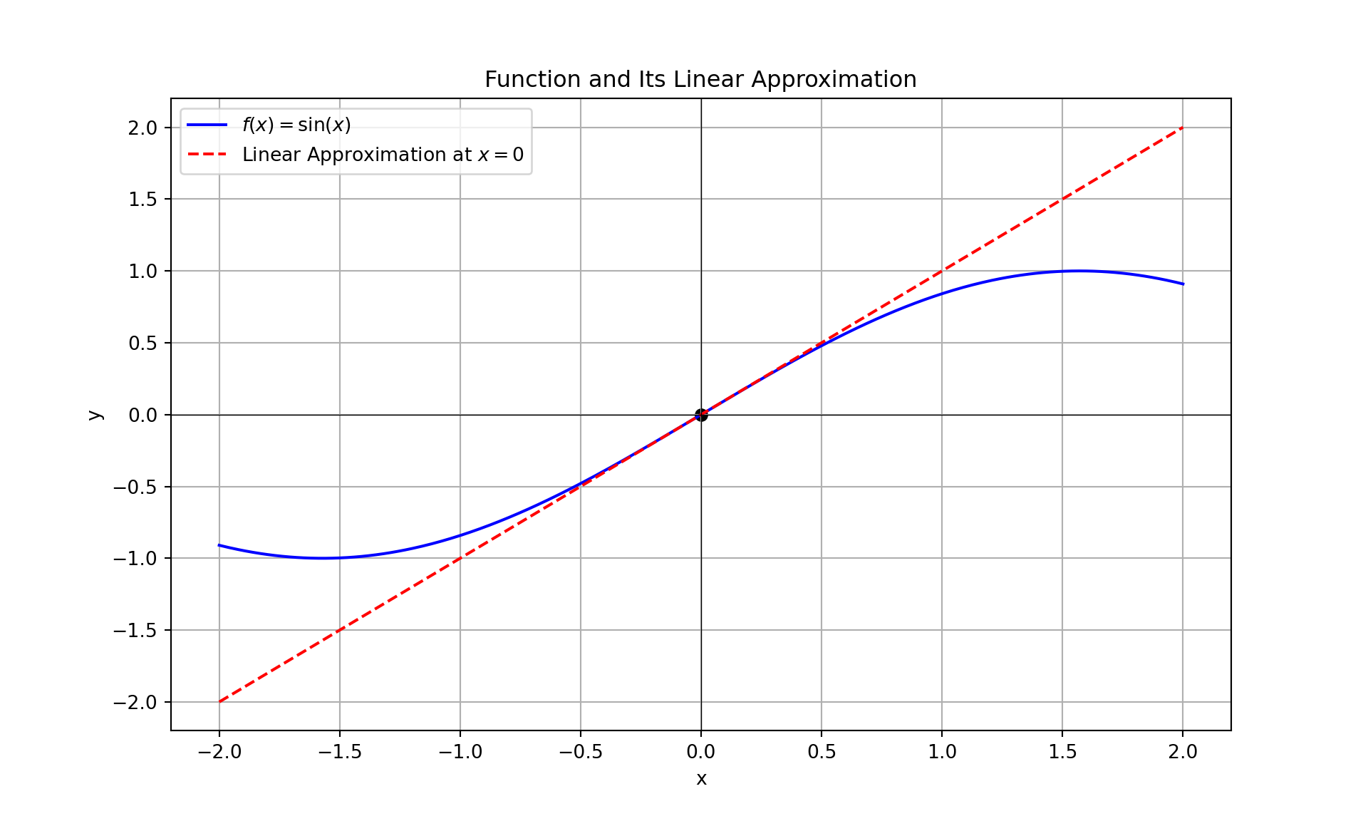

plt.show()

3.6.8.1 Problems and Solutions- Linearization of Functions

Find the linearization of the following functions at the point specified.

1. Function: \(f(x) = x^2\) Point: \(x = 3\)

2. Function: \(f(x) = \sqrt{x}\) Point: \(x = 4\)

3. Function: \(f(x) = \ln(x)\) Point: \(x = 1\)

4. Function: \(f(x) = e^x\) Point: \(x = 0\)

5. Function: \(f(x) = \sin(x)\) Point: \(x = \frac{\pi}{4}\)

6. Function: \(f(x) = \frac{1}{x}\) Point: \(x = 2\)

7. Function: \(f(x) = \tan(x)\) Point: \(x = 0\)

8. Function: \(f(x) = \cos(x)\) Point: \(x = \frac{\pi}{3}\)

9. Function: \(f(x) = x^3 - 2x\) Point: \(x = 1\)

10. Function: \(f(x) = \frac{\sqrt{x}}{x + 1}\) Point: \(x = 1\)

---

Solutions

Problem 1: Function: \(f(x) = x^2\) at \(x = 3\).

1. Find the derivative: \[ f'(x) = 2x \]

2. Evaluate at \(x = 3\): \[ f'(3) = 2 \cdot 3 = 6 \]

3. Linearization formula: \[ \begin{align*} L(x) &= f(3) + f'(3) \cdot (x - 3) \\ &= 3^2 + 6 \cdot (x - 3) \\ &= 9 + 6(x - 3) \\ &= 6x - 9 \end{align*} \]

---

Problem 2: Function: \(f(x) = \sqrt{x}\) at \(x = 4\).

1. Find the derivative: \[ f'(x) = \frac{1}{2\sqrt{x}} \]

2. Evaluate at \(x = 4\): \[ f'(4) = \frac{1}{2 \cdot \sqrt{4}} = \frac{1}{4} \]

3. Linearization formula: \[ \begin{align*} L(x) &= f(4) + f'(4) \cdot (x - 4) \\ &= \sqrt{4} + \frac{1}{4} \cdot (x - 4) \\ &= 2 + \frac{1}{4}(x - 4) \\ &= \frac{1}{4}x + 1 \end{align*} \]

---

Problem 3: Function: \(f(x) = \ln(x)\) at \(x = 1\).

1. Find the derivative: \[ f'(x) = \frac{1}{x} \]

2. Evaluate at \(x = 1\): \[ f'(1) = \frac{1}{1} = 1 \]

3. Linearization formula: \[ \begin{align*} L(x) &= f(1) + f'(1) \cdot (x - 1) \\ &= \ln(1) + 1 \cdot (x - 1) \\ &= 0 + (x - 1) \\ &= x - 1 \end{align*} \]

---

Problem 4: Function: \(f(x) = e^x\) at \(x = 0\).

1. Find the derivative: \[ f'(x) = e^x \]

2. Evaluate at \(x = 0\): \[ f'(0) = e^0 = 1 \]

3. Linearization formula: \[ \begin{align*} L(x) &= f(0) + f'(0) \cdot (x - 0) \\ &= e^0 + 1 \cdot x \\ &= 1 + x \end{align*} \]

---

Problem 5: Function: \(f(x) = \sin(x)\) at \(x = \frac{\pi}{4}\).

1. Find the derivative: \[ f'(x) = \cos(x) \]

2. Evaluate at \(x = \frac{\pi}{4}\): \[ f'\left(\frac{\pi}{4}\right) = \cos\left(\frac{\pi}{4}\right) = \frac{\sqrt{2}}{2} \]

3. Linearization formula: \[ \begin{align*} L(x) &= f\left(\frac{\pi}{4}\right) + f'\left(\frac{\pi}{4}\right) \cdot \left(x - \frac{\pi}{4}\right) \\ &= \sin\left(\frac{\pi}{4}\right) + \frac{\sqrt{2}}{2} \cdot \left(x - \frac{\pi}{4}\right) \\ &= \frac{\sqrt{2}}{2} + \frac{\sqrt{2}}{2} \cdot \left(x - \frac{\pi}{4}\right) \end{align*} \]

---

Problem 6: Function: \(f(x) = \frac{1}{x}\) at \(x = 2\).

1. Find the derivative: \[ f'(x) = -\frac{1}{x^2} \]

2. Evaluate at \(x = 2\): \[ f'(2) = -\frac{1}{2^2} = -\frac{1}{4} \]

3. Linearization formula: \[ \begin{align*} L(x) &= f(2) + f'(2) \cdot (x - 2) \\ &= \frac{1}{2} - \frac{1}{4} \cdot (x - 2) \\ &= \frac{1}{2} - \frac{1}{4}x + \frac{1}{2} \\ &= 1 - \frac{1}{4}x \end{align*} \]

---

Problem 7: Function: \(f(x) = \tan(x)\) at \(x = 0\).

1. Find the derivative: \[ f'(x) = \sec^2(x) \]

2. Evaluate at \(x = 0\): \[ f'(0) = \sec^2(0) = 1 \]

3. Linearization formula: \[ \begin{align*} L(x) &= f(0) + f'(0) \cdot (x - 0) \\ &= \tan(0) + 1 \cdot x \\ &= 0 + x \\ &= x \end{align*} \]

---

Problem 8: Function: \(f(x) = \cos(x)\) at \(x = \frac{\pi}{3}\).

1. Find the derivative: \[ f'(x) = -\sin(x) \]

2. Evaluate at \(x = \frac{\pi}{3}\): \[ f'\left(\frac{\pi}{3}\right) = -\sin\left(\frac{\pi}{3}\right) = -\frac{\sqrt{3}}{2} \]

3. Linearization formula: \[ \begin{align*} L(x) &= f\left(\frac{\pi}{3}\right) + f'\left(\frac{\pi}{3}\right) \cdot \left(x - \frac{\pi}{3}\right) \\ &= \cos\left(\frac{\pi}{3}\right) - \frac{\sqrt{3}}{2} \cdot \left(x - \frac{\pi}{3}\right) \\ &= \frac{1}{2} - \frac{\sqrt{3}}{2} \cdot \left(x - \frac{\pi}{3}\right) \end{align*} \]

---

Problem 9: Function: \(f(x) = x^3 - 2x\) at \(x = 1\).

1. Find the derivative: \[ f'(x) = 3x^2 - 2 \]

2. Evaluate at \(x = 1\): \[ f'(1) = 3 \cdot 1^2 - 2 = 1 \]

3. Linearization formula: \[ \begin{align*} L(x) &= f(1) + f'(1) \cdot (x - 1) \\ &= (1^3 - 2 \cdot 1) + 1 \cdot (x - 1) \\ &= -1 + (x - 1) \\ &= x - 2 \end{align*} \]

---

Problem 10: Function \(f(x) = \frac{\sqrt{x}}{x + 1}\) at \(x = 1\).

1. Find the derivative: \[ f'(x) = \frac{\frac{1 + 1}{2 \cdot \sqrt{x}} \cdot (x + 1) - \sqrt{x}}{(x + 1)^2} \]

2. Evaluate at \(x = 1\): \[ f'(1) = \frac{\frac{1 + 1}{2 \cdot \sqrt{1}} - \sqrt{1}}{(1 + 1)^2} = \frac{1 - 1}{4} = 0 \]

3. Linearization formula: \[ \begin{align*} L(x) &= f(1) + f'(1) \cdot (x - 1) \\ &= \frac{\sqrt{1}}{1 + 1} + 0 \cdot (x - 1) \\ &= \frac{1}{2} \end{align*} \]

3.6.9 Extending from First Derivatives to Higher-Order Derivatives

First Derivative Recap

In the previous sections, we explored the concept of the first derivative. Recall that the first derivative of a function \(f(x)\), denoted as \(f'(x)\) or \(\frac{d}{dx}[f(x)]\), provides the rate of change of the function at any given point. It represents the slope of the tangent line to the function’s graph at that point. Mathematically, the first derivative is defined as:

\[ f'(x) = \lim_{h \to 0} \frac{f(x + h) - f(x)}{h} \]

The first derivative is crucial because it gives us information about the function’s behavior, such as where it is increasing or decreasing and where it has critical points (local maxima and minima).

3.6.9.1 Second-Order Derivative

To gain deeper insights into a function’s behavior, we look at the second derivative, which is the derivative of the first derivative. It is denoted as \(f''(x)\) or \(\frac{d^2}{dx^2}[f(x)]\). The second derivative provides information about the curvature or concavity of the function’s graph.

Mathematical Definition:

\[ f''(x) = \frac{d}{dx}[f'(x)] = \lim_{h \to 0} \frac{f'(x + h) - f'(x)}{h} \]

Geometric Implications:

• Concavity: The second derivative reveals how the function is curving:
  • If \(f''(x) > 0\), the function is concave up at that point. This means the graph is bending upwards, and the tangent line is below the curve.
  • If \(f''(x) < 0\), the function is concave down at that point. This means the graph is bending downwards, and the tangent line is above the curve.
• Points of Inflection: A point where the second derivative changes sign is called a point of inflection. At such points, the graph of the function changes its concavity. For instance:
  • If a function changes from concave up to concave down at a point, that point is a point of inflection.
  • Conversely, if it changes from concave down to concave up, it is also a point of inflection.

Visualizing Concavity:

• When the second derivative is positive, the graph of the function has a “U” shape in the local region, which is often described as “smiling.”
• When the second derivative is negative, the graph has an “n” shape, described as “frowning.”

3.6.9.2 Higher-Order Derivatives

Beyond the second derivative, we can compute higher-order derivatives, which are the derivatives of the second derivative, third derivative, and so on. These derivatives are denoted as \(f'''(x)\), \(f^{(4)}(x)\), etc., and provide further insight into the function’s behavior.

Mathematical Definition:

For the third derivative: \[ f'''(x) = \frac{d}{dx}[f''(x)] \]

For the fourth derivative: \[ f^{(4)}(x) = \frac{d}{dx}[f'''(x)] \]

Significance:

• Rate of Change of Curvature: Higher-order derivatives help in understanding the rate at which the curvature itself is changing. This is particularly useful in physics and engineering for modeling complex motion or forces.
• Taylor Series Expansion: Higher-order derivatives are used in Taylor series to approximate functions locally by polynomials, providing a powerful tool for numerical methods and simulations.

Applications in Computer Science and Engineering:

1. Computer Graphics: In computer graphics, the second derivative is used to calculate surface curvature, which helps in rendering smooth surfaces and textures. For instance, in shading and rendering, knowing how the surface curves can influence light reflection and shading techniques.

2. Machine Learning: In optimization algorithms such as Newton’s method, higher-order derivatives are used to find local minima or maxima more efficiently by considering not just the slope but also the curvature of the cost function.

3. Animation: For creating realistic animations, understanding how motion changes over time (through second and higher-order derivatives) helps in producing smooth and natural movements. For example, in physics-based animation, the second derivative (acceleration) is crucial for accurately simulating the effects of forces.

While the first derivative provides the basic rate of change and slope of a function, the second derivative reveals the function’s curvature and concavity, and higher-order derivatives offer insights into more complex behaviors. These derivatives are essential tools for understanding and analyzing functions in various applications, including computer science, engineering, and beyond.

3.6.9.3 Example: Analyzing Curvature and Points of Inflection

In this example, we use the function \(f(x) = x^3 - 3x^2 + 2\) to illustrate how the first and second derivatives help in understanding the behavior of the function, particularly focusing on concavity and points of inflection.

Mathematical Model (Cubic Spline):

• Function: \(f(x) = x^3 - 3x^2 + 2\)
• First Derivative: \(f'(x) = 3x^2 - 6x\)
• Second Derivative: \(f''(x) = 6x - 6\)

Python Code for Visualization

import numpy as np
import matplotlib.pyplot as plt

# Define the function and its derivatives
def f(x):
    return x**3 - 3*x**2 + 2

def f_prime(x):
    return 3*x**2 - 6*x

def f_double_prime(x):
    return 6*x - 6

# Define the x values
x = np.linspace(-1, 4, 400)
y = f(x)
y_prime = f_prime(x)
y_double_prime = f_double_prime(x)

# Create a figure with multiple subplots
plt.figure(figsize=(14, 10))

## <Figure size 1400x1000 with 0 Axes>

# Plot the function
plt.plot(x, y, label='$f(x) = x^3 - 3x^2 + 2$', color='blue', linewidth=2)

## [<matplotlib.lines.Line2D object at 0x0000029F569E48B0>]

# Plot the first derivative
plt.plot(x, y_prime, label="$f'(x) = 3x^2 - 6x$", color='green', linestyle='--')

## [<matplotlib.lines.Line2D object at 0x0000029F57012820>]

# Plot the second derivative
plt.plot(x, y_double_prime, label="$f''(x) = 6x - 6$", color='red', linestyle=':')

## [<matplotlib.lines.Line2D object at 0x0000029F567136A0>]

# Highlight points of inflection where second derivative changes sign
inflection_points_x = [1]
inflection_points_y = [f(1)]
plt.scatter(inflection_points_x, inflection_points_y, color='black', zorder=5, label='Point of Inflection')

## <matplotlib.collections.PathCollection object at 0x0000029F56A01130>

# Annotate the plot
plt.title('Function and Its Derivatives')

## Text(0.5, 1.0, 'Function and Its Derivatives')

plt.xlabel('x')

## Text(0.5, 0, 'x')

plt.ylabel('y')

## Text(0, 0.5, 'y')

plt.axhline(0, color='black',linewidth=0.5)

## <matplotlib.lines.Line2D object at 0x0000029F569E4070>

plt.axvline(0, color='black',linewidth=0.5)

## <matplotlib.lines.Line2D object at 0x0000029F56713AF0>

plt.grid(True)
plt.legend()

## <matplotlib.legend.Legend object at 0x0000029F56D9BDC0>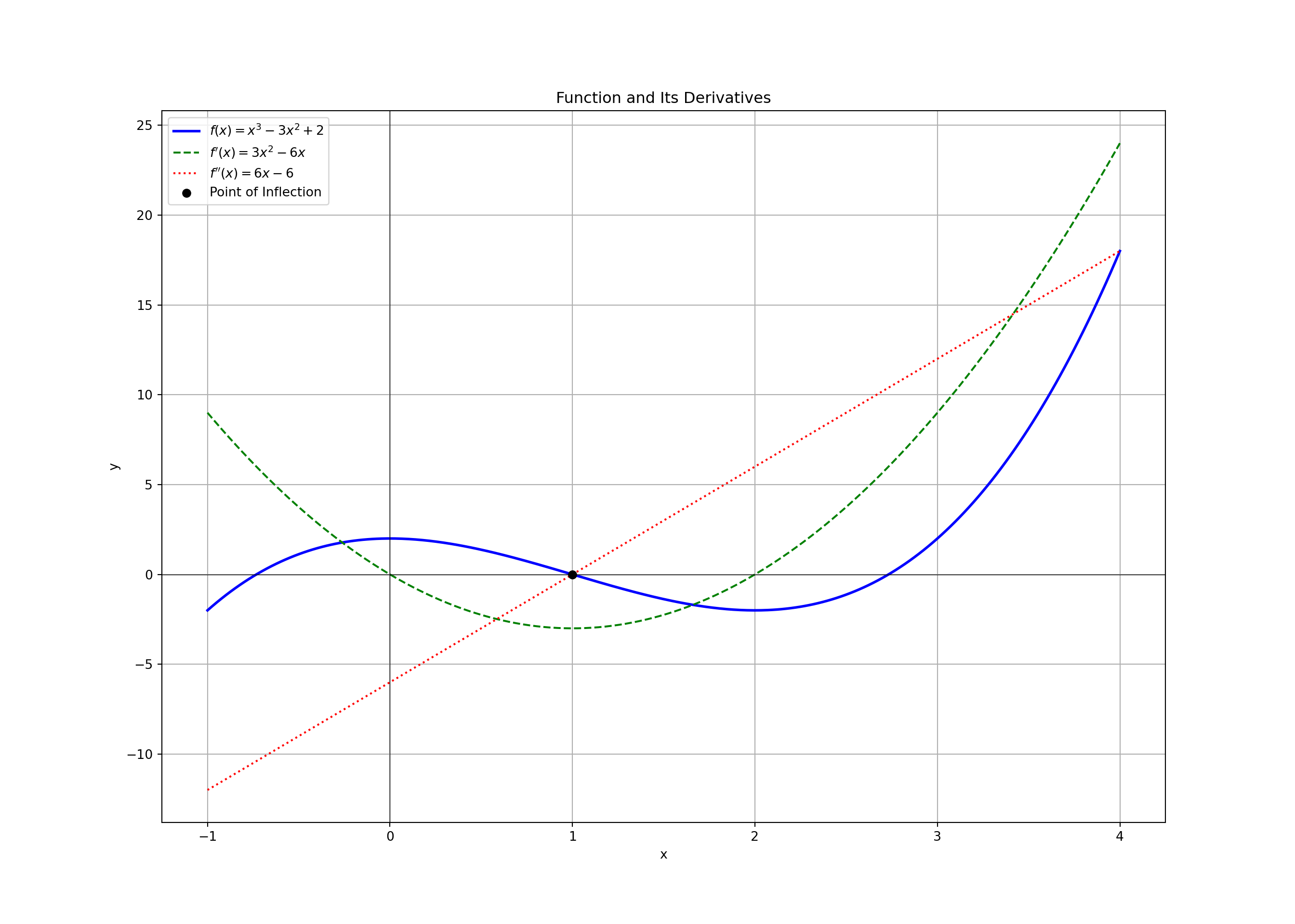

plt.show()

Interpretation of various graphs in the plot

1. Function \(f(x) = x^3 - 3x^2 + 2\) (Blue Line): - This graph represents the function whose behavior is being analyzed. It has a cubic shape with local maxima and minima.

2. First Derivative \(f'(x) = 3x^2 - 6x\) (Green Dashed Line): Shows the rate of change of the function \(f(x)\). The x-intercepts of this graph (i.e., where \(f'(x) = 0\)) are the critical points where the function may have local maxima or minima: At \(x = 0\): This is a local minimum because the function changes from decreasing to increasing at this point. At \(x = 2\): This is a local maximum because the function changes from increasing to decreasing at this point.

3. Second Derivative \(f''(x) = 6x - 6\) (Red Dotted Line): Reveals the concavity of the function \(f(x)\). Where \(f''(x) > 0\) (i.e., where the red line is above the x-axis), the function is concave up (U-shape). Where \(f''(x) < 0\) (i.e., where the red line is below the x-axis), the function is concave down (n-shape). The x-intercept at \(x = 1\) is the point of inflection, where the concavity of the function changes.

4. Point of Inflection (Black Dot): The point of inflection is at \(x = 1\), where the function changes from concave down to concave up. At this point, the second derivative \(f''(x)\) crosses the x-axis, indicating a change in the curvature of the function.

Note: By analyzing the function along with its first and second derivatives, we can gain a comprehensive understanding of its behavior, including local extrema and changes in concavity. This holistic view is crucial for tasks like optimization, curve fitting, and understanding the overall shape of functions in computer science and engineering applications.

3.6.9.4 Problems on Higher-Order Derivatives

Problems

Second Order Derivatives

Problem 1:
Find the second derivative of \(f(x) = x^3 + 3x^2 + 2x + 1\).

---

Problem 2:
Find the second derivative of \(f(x) = e^{2x}\).

---

Problem 3:
Find the second derivative of \(f(x) = \sin(x)\).

---

Problem 4:
Find the second derivative of \(f(x) = \ln(x)\).

---

Problem 5:
Find the second derivative of \(f(x) = \cosh(x)\).

---

Third Order Derivatives

Problem 1:
Find the third derivative of \(f(x) = x^4 - 2x^3 + x - 1\).

---

Problem 2:
Find the third derivative of \(f(x) = e^{3x}\).

---

Problem 3:
Find the third derivative of \(f(x) = \sin(x)\).

---

Problem 4:
Find the third derivative of \(f(x) = \ln(x)\).

---

Problem 5:
Find the third derivative of \(f(x) = \tanh(x)\).

---

Fourth Order Derivatives

Problem 1:
Find the fourth derivative of \(f(x) = x^5 - 4x^4 + x^2 - x + 1\).

---

Problem 2:
Find the fourth derivative of \(f(x) = e^{4x}\).

---

Problem 3:
Find the fourth derivative of \(f(x) = \sin(x)\).

---

Problem 4:
Find the fourth derivative of \(f(x) = \ln(x)\).

---

Problem 5:
Find the fourth derivative of \(f(x) = \text{sech}(x)\).

---

Solutions

Second Order Derivatives

Solution 1:
Find the second derivative of \(f(x) = x^3 + 3x^2 + 2x + 1\).

1. First Derivative: \[ f'(x) = 3x^2 + 6x + 2 \]

2. Second Derivative: \[ f''(x) = 6x + 6 \]

---

Solution 2:
Find the second derivative of \(f(x) = e^{2x}\).

1. First Derivative: \[ f'(x) = 2e^{2x} \]

2. Second Derivative: \[ f''(x) = 4e^{2x} \]

---

Solution 3:
Find the second derivative of \(f(x) = \sin(x)\).

1. First Derivative: \[ f'(x) = \cos(x) \]

2. Second Derivative: \[ f''(x) = -\sin(x) \]

---

Solution 4:
Find the second derivative of \(f(x) = \ln(x)\).

1. First Derivative: \[ f'(x) = \frac{1}{x} \]

2. Second Derivative: \[ f''(x) = -\frac{1}{x^2} \]

---

Solution 5:
Find the second derivative of \(f(x) = \cosh(x)\).

1. First Derivative: \[ f'(x) = \sinh(x) \]

2. Second Derivative: \[ f''(x) = \cosh(x) \]

---

Third Order Derivatives

Solution 1:
Find the third derivative of \(f(x) = x^4 - 2x^3 + x - 1\).

1. First Derivative: \[ f'(x) = 4x^3 - 6x^2 + 1 \]

2. Second Derivative: \[ f''(x) = 12x^2 - 12x \]

3. Third Derivative: \[ f'''(x) = 24x - 12 \]

---

Solution 2:
Find the third derivative of \(f(x) = e^{3x}\).

1. First Derivative: \[ f'(x) = 3e^{3x} \]

2. Second Derivative: \[ f''(x) = 9e^{3x} \]

3. Third Derivative: \[ f'''(x) = 27e^{3x} \]

---

Solution 3:
Find the third derivative of \(f(x) = \sin(x)\).

1. First Derivative: \[ f'(x) = \cos(x) \]

2. Second Derivative: \[ f''(x) = -\sin(x) \]

3. Third Derivative: \[ f'''(x) = -\cos(x) \]

---

Solution 4:
Find the third derivative of \(f(x) = \ln(x)\).

1. First Derivative: \[ f'(x) = \frac{1}{x} \]

2. Second Derivative: \[ f''(x) = -\frac{1}{x^2} \]

3. Third Derivative: \[ f'''(x) = \frac{2}{x^3} \]

---

Solution 5:
Find the third derivative of \(f(x) = \tanh(x)\).

1. First Derivative: \[ f'(x) = \text{sech}^2(x) \]

2. Second Derivative: \[ f''(x) = -2 \text{sech}^2(x) \tanh(x) \]

3. Third Derivative: \[ f'''(x) = 2 \text{sech}^2(x) \left(2\tanh^2(x) - \text{sech}^2(x)\right) \]

---

Fourth Order Derivatives

Solution 1:
Find the fourth derivative of \(f(x) = x^5 - 4x^4 + x^2 - x + 1\).

1. First Derivative: \[ f'(x) = 5x^4 - 16x^3 + 2x - 1 \]

2. Second Derivative: \[ f''(x) = 20x^3 - 48x^2 + 2 \]

3. Third Derivative: \[ f'''(x) = 60x^2 - 96x \]

4. Fourth Derivative: \[ f''''(x) = 120x - 96 \]

---

Solution 2:
Find the fourth derivative of \(f(x) = e^{4x}\).

1. First Derivative: \[ f'(x) = 4e^{4x} \]

2. Second Derivative: \[ f''(x) = 16e^{4x} \]

3. Third Derivative: \[ f'''(x) = 64e^{4x} \]

4. Fourth Derivative: \[ f''''(x) = 256e^{4x} \]

---

Solution 3:
Find the fourth derivative of \(f(x) = \sin(x)\).

1. First Derivative: \[ f'(x) = \cos(x) \]

2. Second Derivative: \[ f''(x) = -\sin(x) \]

3. Third Derivative: \[ f'''(x) = -\cos(x) \]

4. Fourth Derivative: \[ f''''(x) = \sin(x) \]

---

Solution 4:
Find the fourth derivative of \(f(x) = \ln(x)\).

1. First Derivative: \[ f'(x) = \frac{1}{x} \]

2. Second Derivative: \[ f''(x) = -\frac{1}{x^2} \]

3. Third Derivative: \[ f'''(x) = \frac{2}{x^3} \]

4. Fourth Derivative: \[ f''''(x) = -\frac{6}{x^4} \]

---

Solution 5:
Find the fourth derivative of \(f(x) = \text{sech}(x)\).

1. First Derivative: \[ f'(x) = -\text{sech}(x) \tanh(x) \]

2. Second Derivative: \[ f''(x) = \text{sech}(x) \left(\text{sech}^2(x) - \tanh^2(x)\right) \]

3. Third Derivative: \[ f'''(x) = -\text{sech}(x) \left(2 \text{sech}^2(x) \tanh(x) - \tanh^3(x) \right) \]

4. Fourth Derivative: \[ f''''(x) = \text{sech}(x) \left( 8\text{sech}^4(x) \tanh(x) - 8\text{sech}^2(x) \tanh^3(x) + \tanh^5(x) - 6\text{sech}^6(x) \right) \]

3.6.9.5 Application-Level Problems Using Higher-Order Derivatives

Problems

Problem 1:
A beam is subjected to a load that causes its deflection to be described by the function \(y(x) = \frac{x^4}{4} - x^3 + 2x^2\). Find the equation of the bending moment \(M(x)\) along the beam.

---

Problem 2:
The position \(s(t)\) of a particle moving along a straight line is given by \(s(t) = t^4 - 4t^3 + 6t^2\). Find the jerk (third derivative of position with respect to time) of the particle at \(t = 2\).

---

Problem 3:
A function \(f(x)\) is given by \(f(x) = x^5 - 10x^3 + 15x\). Determine the points of inflection for this function.

---

Problem 4:
The temperature distribution along a rod at time \(t\) is given by \(T(x,t) = e^{-t}(x^2 + 4x + 5)\). Find the second derivative of temperature with respect to position \(x\) and interpret its physical meaning.

---

Problem 5:
The electric potential \(V\) in a region of space is given by \(V(x,y) = x^4 + y^4 - 4x^2y^2\). Determine the points where the second derivatives of \(V\) with respect to \(x\) and \(y\) are zero.

---

Solutions

Solution 1:
A beam is subjected to a load that causes its deflection to be described by the function \(y(x) = \frac{x^4}{4} - x^3 + 2x^2\). Find the equation of the bending moment \(M(x)\) along the beam.

1. Find the first derivative \(y'(x)\): \[ y'(x) = x^3 - 3x^2 + 4x \]

2. Find the second derivative \(y''(x)\): \[ y''(x) = 3x^2 - 6x + 4 \]

3. The bending moment \(M(x)\) is proportional to the second derivative of deflection: \[ M(x) \propto y''(x) \]

4. Therefore, the equation of the bending moment \(M(x)\) is: \[ M(x) = C (3x^2 - 6x + 4) \] where \(C\) is a constant of proportionality.

---

Solution 2:
The position \(s(t)\) of a particle moving along a straight line is given by \(s(t) = t^4 - 4t^3 + 6t^2\). Find the jerk (third derivative of position with respect to time) of the particle at \(t = 2\).

1. Find the first derivative \(s'(t)\) (velocity): \[ s'(t) = 4t^3 - 12t^2 + 12t \]

2. Find the second derivative \(s''(t)\) (acceleration): \[ s''(t) = 12t^2 - 24t + 12 \]

3. Find the third derivative \(s'''(t)\) (jerk): \[ s'''(t) = 24t - 24 \]

4. Evaluate the jerk at \(t = 2\): \[ s'''(2) = 24(2) - 24 = 48 - 24 = 24 \]

5. Therefore, the jerk at \(t = 2\) is: \[ s'''(2) = 24 \, \text{units/s}^3 \]

---

Solution 3:
A function \(f(x)\) is given by \(f(x) = x^5 - 10x^3 + 15x\). Determine the points of inflection for this function.

1. Find the first derivative \(f'(x)\): \[ f'(x) = 5x^4 - 30x^2 + 15 \]

2. Find the second derivative \(f''(x)\): \[ f''(x) = 20x^3 - 60x \]

3. Find the third derivative \(f'''(x)\): \[ f'''(x) = 60x^2 - 60 \]

4. Set the second derivative to zero and solve for \(x\): \[ 20x^3 - 60x = 0 \] \[ 20x(x^2 - 3) = 0 \] \[ x = 0, \pm \sqrt{3} \]

5. Determine the concavity change around these points to confirm inflection points:

   • For \(x = 0\): \(f''(x) = 0\)
   • For \(x = \sqrt{3}\) and \(x = -\sqrt{3}\): Check the sign change in \(f''(x)\)

6. Therefore, the points of inflection are: \[ x = 0, \sqrt{3}, -\sqrt{3} \]

---

Solution 4:
The temperature distribution along a rod at time \(t\) is given by \(T(x,t) = e^{-t}(x^2 + 4x + 5)\). Find the second derivative of temperature with respect to position \(x\) and interpret its physical meaning.

1. Find the first derivative \(T_x(x,t)\) with respect to \(x\): \[ T_x(x,t) = e^{-t}(2x + 4) \]

2. Find the second derivative \(T_{xx}(x,t)\) with respect to \(x\): \[ T_{xx}(x,t) = e^{-t}(2) \]

3. Interpretation: \[ T_{xx}(x,t) = 2e^{-t} \] The second derivative of temperature with respect to position \(x\) indicates the rate of change of the temperature gradient along the rod. Since \(T_{xx}(x,t)\) is constant in \(x\), it suggests a uniform concavity in the temperature profile along the rod.

---

Solution 5:
The electric potential \(V\) in a region of space is given by \(V(x,y) = x^4 + y^4 - 4x^2y^2\). Determine the points where the second derivatives of \(V\) with respect to \(x\) and \(y\) are zero.

1. Find the second derivative \(V_{xx}\) with respect to \(x\): \[ V_{xx} = 12x^2 - 8y^2 \]

2. Find the second derivative \(V_{yy}\) with respect to \(y\): \[ V_{yy} = 12y^2 - 8x^2 \]

3. Set both second derivatives to zero and solve for \(x\) and \(y\):

   • For \(V_{xx} = 0\): \[ 12x^2 - 8y^2 = 0 \] \[ 3x^2 = 2y^2 \] \[ x = \pm \sqrt{\frac{2}{3}}y \]

   • For \(V_{yy} = 0\): \[ 12y^2 - 8x^2 = 0 \] \[ 3y^2 = 2x^2 \] \[ y = \pm \sqrt{\frac{2}{3}}x \]

4. Combine the results: \[ x = 0, y = 0 \quad \text{and} \quad x = \pm \sqrt{\frac{2}{3}}y, y = \pm \sqrt{\frac{2}{3}}x \]

5. Therefore, the points where the second derivatives are zero are: \[ (0,0), \left(\sqrt{\frac{2}{3}}, \sqrt{\frac{2}{3}}\right), \left(-\sqrt{\frac{2}{3}}, \sqrt{\frac{2}{3}}\right), \left(\sqrt{\frac{2}{3}}, -\sqrt{\frac{2}{3}}\right), \left(-\sqrt{\frac{2}{3}}, -\sqrt{\frac{2}{3}}\right) \]

3.6.10 Convexity and Concavity of Functions

Understanding the concepts of convexity and concavity helps in various fields, such as optimization, economics, and machine learning, where the nature of functions plays a crucial role in finding optimal solutions and modeling behaviors.

Intuitive Definitions

Convexity: A function \(f(x)\) is convex on an interval if, for any two points \(x_1\) and \(x_2\) within the interval, the line segment joining the points \((x_1, f(x_1))\) and \((x_2, f(x_2))\) lies above the graph of the function. In simpler terms, a function is convex if it “bends upwards” and has a shape like the bowl of a spoon.

Concavity: A function \(f(x)\) is concave on an interval if, for any two points \(x_1\) and \(x_2\) within the interval, the line segment joining the points \((x_1, f(x_1))\) and \((x_2, f(x_2))\) lies below the graph of the function. In simpler terms, a function is concave if it “bends downwards” and has a shape like the inverted bowl.

Mathematical Tools to Investigate Convexity and Concavity

First Derivative Test: To determine if a function is convex or concave, the first derivative test involves checking whether the function is increasing or decreasing.

1. Function is Convex:
   • If the first derivative \(f'(x)\) is increasing, then \(f(x)\) is convex.
   • This means that the slope of the function is getting steeper.
2. Function is Concave:
   • If the first derivative \(f'(x)\) is decreasing, then \(f(x)\) is concave.
   • This means that the slope of the function is getting shallower.

Second Derivative Test: A more direct method involves using the second derivative of the function.

1. Function is Convex:
   • If the second derivative \(f''(x)\) is positive for all \(x\) in the interval, then \(f(x)\) is convex on that interval.
2. Function is Concave:
   • If the second derivative \(f''(x)\) is negative for all \(x\) in the interval, then \(f(x)\) is concave on that interval.

Mathematical Notations

1. Convex Function: \[ f''(x) > 0 \]

2. Concave Function: \[ f''(x) < 0 \]

Example: Consider the function \(f(x) = x^3 - 3x^2 + 2\).

Analyzing Convexity and Concavity

1. Find the First Derivative: \[ f'(x) = 3x^2 - 6x \]

2. Find the Second Derivative: \[ f''(x) = 6x - 6 \]

3. Determine the Sign of the Second Derivative:

   • For \(x > 1\), \(f''(x) > 0\), so \(f(x)\) is convex.
   • For \(x < 1\), \(f''(x) < 0\), so \(f(x)\) is concave.

Note: By plotting the function \(f(x) = x^3 - 3x^2 + 2\), we can visualize how the function changes from being concave to convex at the point where the second derivative changes sign. The point where \(f''(x) = 0\) is called the inflection point, where the function transitions from concavity to convexity.

3.6.10.1 Problems on Concavity and Convexity of Functions

Problems

Problem 1: \(f(x) = x^2\) in the interval, \((-\infty, \infty)\).

Problem 2: \(f(x) = -x^2 + 4x + 1\) in the interval \((-\infty, \infty)\).

Problem 3: \(f(x) = e^x\) in the interval \((-\infty, \infty)\).

Problem 4: \(f(x) = \ln(x)\) in the interval \((0, \infty)\).

Problem 5: \(f(x) = \sqrt{x}\) in the interval \((0, \infty)\).

*Problem 6:** \(f(x) = x^3 - 3x\) in the interval \((-\infty, \infty)\).

Problem 7: \(f(x) = \frac{1}{x^2}\) in the interval \((0, \infty)\).

Problem 8: \(f(x) = \sin(x)\) in the interval \((0, \pi)\).

Problem 9: \(f(x) = x^4 - 4x^2\)in the interval \((-\infty, \infty)\).

Problem 10: \(f(x) = \frac{x}{x^2 + 1}\) in the interval \((-\infty, \infty)\).

---

Solutions

Solution 1
Function: \(f(x) = x^2\)
Interval: \((-\infty, \infty)\)

1. Find the Second Derivative: \[ f''(x) = 2 \]

2. Determine Convexity/Concavity: \[ f''(x) = 2 > 0 \] Since \(f''(x) > 0\), the function \(f(x)\) is convex.

---

Solution 2
Function: \(f(x) = -x^2 + 4x + 1\)
Interval: \((-\infty, \infty)\)

1. Find the Second Derivative: \[ f''(x) = -2 \]

2. Determine Convexity/Concavity: \[ f''(x) = -2 < 0 \] Since \(f''(x) < 0\), the function \(f(x)\) is concave.

---

Solution 3
Function: \(f(x) = e^x\)
Interval: \((-\infty, \infty)\)

1. Find the Second Derivative: \[ f''(x) = e^x \]

2. Determine Convexity/Concavity: \[ f''(x) = e^x > 0 \] Since \(f''(x) > 0\) for all \(x\), the function \(f(x)\) is convex.

---

Solution 4
Function: \(f(x) = \ln(x)\)
Interval: \((0, \infty)\)

1. Find the Second Derivative: \[ f''(x) = -\frac{1}{x^2} \]

2. Determine Convexity/Concavity: \[ f''(x) = -\frac{1}{x^2} < 0 \] Since \(f''(x) < 0\) for \(x > 0\), the function \(f(x)\) is concave.

---

Solution 5
Function: \(f(x) = \sqrt{x}\)
Interval: \((0, \infty)\)

1. Find the Second Derivative: \[ f''(x) = -\frac{1}{4}x^{-\frac{3}{2}} \]

2. Determine Convexity/Concavity: \[ f''(x) = -\frac{1}{4}x^{-\frac{3}{2}} < 0 \] Since \(f''(x) < 0\) for \(x > 0\), the function \(f(x)\) is concave.

---

Solution 6
Function: \(f(x) = x^3 - 3x\)
Interval: \((-\infty, \infty)\)

1. Find the Second Derivative: \[ f''(x) = 6x \]

2. Determine Convexity/Concavity:

   • For \(x > 0\), \(f''(x) > 0\), so \(f(x)\) is convex.
   • For \(x < 0\), \(f''(x) < 0\), so \(f(x)\) is concave.

---

Solution 7
Function: \(f(x) = \frac{1}{x^2}\)
Interval: \((0, \infty)\)

1. Find the Second Derivative: \[ f''(x) = \frac{6}{x^4} \]

2. Determine Convexity/Concavity: \[ f''(x) = \frac{6}{x^4} > 0 \] Since \(f''(x) > 0\) for \(x > 0\), the function \(f(x)\) is convex.

---

Solution 8
Function: \(f(x) = \sin(x)\)
Interval: \((0, \pi)\)

1. Find the Second Derivative: \[ f''(x) = -\sin(x) \]

2. Determine Convexity/Concavity:

   • For \(0 < x < \frac{\pi}{2}\), \(f''(x) < 0\), so \(f(x)\) is concave.
   • For \(\frac{\pi}{2} < x < \pi\), \(f''(x) > 0\), so \(f(x)\) is convex.

---

Solution 9
Function: \(f(x) = x^4 - 4x^2\)
Interval: \((-\infty, \infty)\)

1. Find the Second Derivative: \[ f''(x) = 12x^2 - 8 \]

2. Determine Convexity/Concavity:

   • For \(x^2 > \frac{2}{3}\), \(f''(x) > 0\), so \(f(x)\) is convex.
   • For \(x^2 < \frac{2}{3}\), \(f''(x) < 0\), so \(f(x)\) is concave.

---

Solution 10
Function: \(f(x) = \frac{x}{x^2 + 1}\)
Interval: \((-\infty, \infty)\)

1. Find the Second Derivative: \[ f''(x) = \frac{2 - 3x^2}{(x^2 + 1)^3} \]

2. Determine Convexity/Concavity:

   • For \(x^2 < \frac{2}{3}\), \(f''(x) > 0\), so \(f(x)\) is convex.
   • For \(x^2 > \frac{2}{3}\), \(f''(x) < 0\), so \(f(x)\) is concave.

3.7 Module-2 Foundations of Multi variable calculus

Syllabus Content: Functions of Several Variables, Graphs, Level Curves, and Contours of Functions of Two Variables, Limits for Functions of Two Variables, Continuity for Functions of Two Variables, Partial Derivatives of a Functions, Second- Order Partial Derivatives.(Total 9 hours)

3.7.1 Introduction

In single-variable calculus, we explored concepts like limits, continuity, derivatives, and their applications. Now, let’s extend these ideas to functions of several variables. Multivariable calculus is crucial for understanding and solving problems in higher dimensions, such as optimization in machine learning, modeling physical systems, and more.

3.7.2 Introduction to Functions of Several Variables

A function of several variables is a function that takes multiple inputs and produces a single output. For example, \(f(x,y)=x^2+y^2\) is a function of two variables, \(x\) and \(y\). Here \(f\) maps a point \((x,y)\) in the plane to a value \(z\) in space.

Example: Temperature Distribution

To illustrate the concept of functions of several variables, let’s consider the example of temperature distribution in a room. The temperature at any point in the room depends on the coordinates of that point. In mathematical terms, the temperature \(T\) is a function of the coordinates \(x\) and \(y\).

Scenario: Temperature as a Function of Coordinates

Imagine a room where the temperature varies based on the location within the room. Let’s denote the temperature at any point \((x, y)\) as \(T(x, y)\). For simplicity, let’s assume the temperature distribution can be modeled by the function:

\[ T(x, y) = 20 + 5x - 3y \]

Where: - \(T\) is the temperature in degrees Celsius. - \(x\) and \(y\) are the coordinates in meters within the room.

Let’s visualize the temperature distribution in the room using Python as a 3D plot:

import numpy as np
import matplotlib.pyplot as plt
from mpl_toolkits.mplot3d import Axes3D

# Define the coordinates
x = np.linspace(0, 5, 100)
y = np.linspace(0, 5, 100)
X, Y = np.meshgrid(x, y)

# Define the temperature function
T = 20 + 5 * X - 3 * Y

# Plot the temperature distribution
fig = plt.figure()
ax = fig.add_subplot(111, projection='3d')
ax.plot_surface(X, Y, T, cmap='coolwarm')

## <mpl_toolkits.mplot3d.art3d.Poly3DCollection object at 0x0000029F57418310>

ax.set_xlabel('x (m)')

## Text(0.5, 0, 'x (m)')

ax.set_ylabel('y (m)')

## Text(0.5, 0.5, 'y (m)')

ax.set_zlabel('Temperature (°C)')

## Text(0.5, 0, 'Temperature (°C)')

ax.set_title('Temperature Distribution in a Room')

## Text(0.5, 0.92, 'Temperature Distribution in a Room')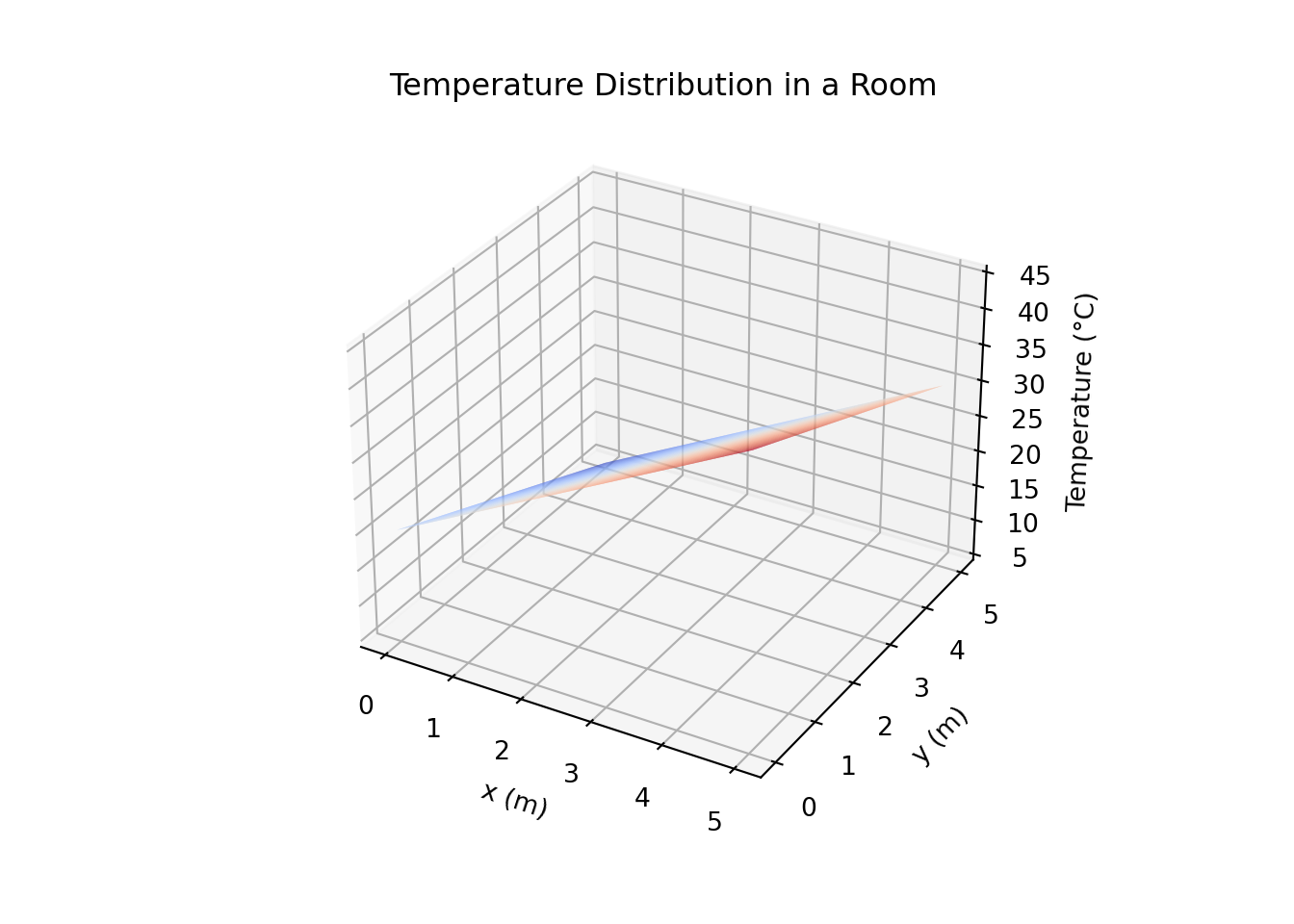

plt.show()

3.7.3 Graph, Level Set (Contours), and Projection of a Function

In multivariable calculus, we often use the concepts of graphs and level sets (contours) to visualize and analyze functions of several variables. Let’s explore these concepts using our temperature distribution example.

Graph: The graph of a function \(T(x, y)\) represents all the points \((x, y, T(x, y))\) in three-dimensional space. For the temperature distribution example, the graph is a surface in 3D space where the height of the surface at any point \((x, y)\) corresponds to the temperature at that point.

Level Set: A level set of a function \(T(x, y)\) is a curve in the \(xy\)-plane where the function has a constant value. For a given constant \(c\), the level set is defined as:

\[ \text{Level Set}(c) = \{ (x, y) \ | \ T(x, y) = c \} \]

For example, if \(T(x, y)\) represents temperature, a level set might represent all the points in a room where the temperature is 25°C.

These level curves help visualize how the function’s value changes across different regions in the \(xy\)-plane, making it easier to analyze the function’s behavior and identify features such as peaks, valleys, and saddle points.

Projection: The projection of the graph of a function \(T(x, y)\) onto the \(xy\)-plane is the shadow or footprint of the 3D graph on the \(xy\)-plane. It shows the \(xy\)-coordinates of all points without considering the value of \(T(x, y)\). This projection helps in understanding the domain of the function and visualizing level sets more effectively.

Let’s visualize the graph and level sets of the above temperature distribution function:

import numpy as np
import matplotlib.pyplot as plt
from mpl_toolkits.mplot3d import Axes3D

# Define the coordinates
x = np.linspace(0, 5, 100)
y = np.linspace(0, 5, 100)
X, Y = np.meshgrid(x, y)

# Define the temperature function
T = 20 + 5 * X - 3 * Y

# Plot the temperature distribution (Graph)
fig = plt.figure(figsize=(12, 6))

# 3D plot for the graph
ax1 = fig.add_subplot(121, projection='3d')
ax1.plot_surface(X, Y, T, cmap='coolwarm')

## <mpl_toolkits.mplot3d.art3d.Poly3DCollection object at 0x0000029F56FFE9A0>

ax1.set_xlabel('x (m)')

## Text(0.5, 0, 'x (m)')

ax1.set_ylabel('y (m)')

## Text(0.5, 0.5, 'y (m)')

ax1.set_zlabel('Temperature (°C)')

## Text(0.5, 0, 'Temperature (°C)')

ax1.set_title('Graph of Temperature Distribution')

## Text(0.5, 0.92, 'Graph of Temperature Distribution')

# 2D contour plot for level sets
ax2 = fig.add_subplot(122)
contour = ax2.contour(X, Y, T, cmap='coolwarm')
ax2.set_xlabel('x (m)')

## Text(0.5, 0, 'x (m)')

ax2.set_ylabel('y (m)')

## Text(0, 0.5, 'y (m)')

ax2.set_title('Level Sets of Temperature Distribution')

## Text(0.5, 1.0, 'Level Sets of Temperature Distribution')

fig.colorbar(contour, ax=ax2, label='Temperature (°C)')

## <matplotlib.colorbar.Colorbar object at 0x0000029F58AD04C0>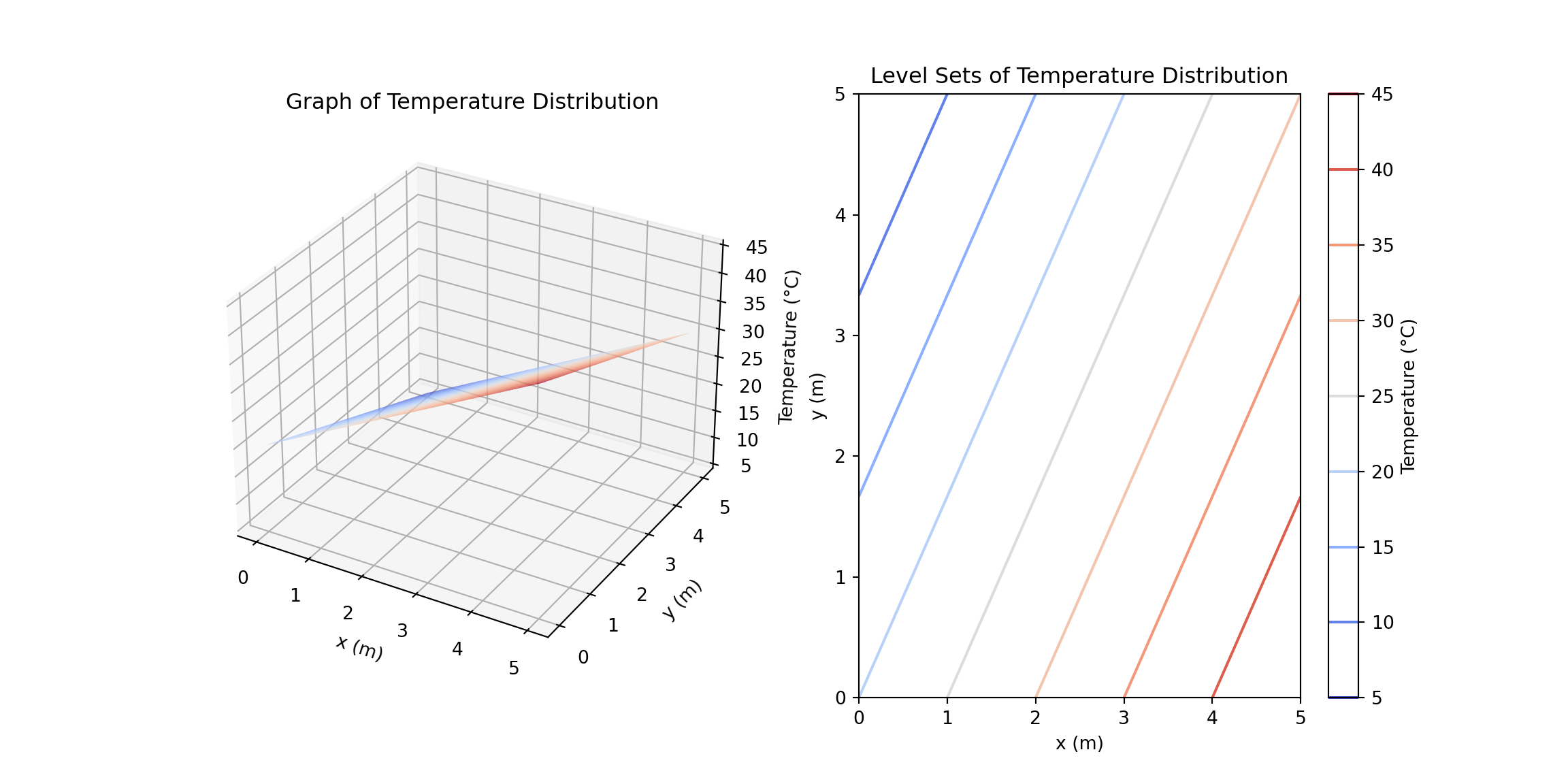

plt.show()

In the following plot, the level sets and projections are visualized:

import numpy as np
import matplotlib.pyplot as plt
from mpl_toolkits.mplot3d import Axes3D

# Define the coordinates
x = np.linspace(0, 5, 100)
y = np.linspace(0, 5, 100)
X, Y = np.meshgrid(x, y)

# Define the temperature function
T = 20 + 5 * X - 3 * Y

# Create the figure and axis object
fig = plt.figure(figsize=(12, 10))
ax = fig.add_subplot(111, projection='3d')

# Plot the temperature distribution (Graph)
surface = ax.plot_surface(X, Y, T, cmap='coolwarm', alpha=0.6, edgecolor='none')

# Plot level sets
contour = ax.contour(X, Y, T, levels=np.linspace(np.min(T), np.max(T), 10), cmap='coolwarm', linestyles='solid', offset=np.min(T) - 10)

# Add projection onto the xy-plane
ax.contourf(X, Y, T, levels=np.linspace(np.min(T), np.max(T), 10), cmap='coolwarm', alpha=0.3)

## <matplotlib.contour.QuadContourSet object at 0x0000029F567FB0A0>

# Adding labels and title
ax.set_xlabel('x (m)')

## Text(0.5, 0, 'x (m)')

ax.set_ylabel('y (m)')

## Text(0.5, 0.5, 'y (m)')

ax.set_zlabel('Temperature (°C)')

## Text(0.5, 0, 'Temperature (°C)')

ax.set_title('Temperature Distribution with Level Sets and Projection')

## Text(0.5, 0.92, 'Temperature Distribution with Level Sets and Projection')

# Add a color bar to show the temperature scale
fig.colorbar(surface, ax=ax, shrink=0.5, aspect=5, label='Temperature (°C)')

## <matplotlib.colorbar.Colorbar object at 0x0000029F5687E3D0>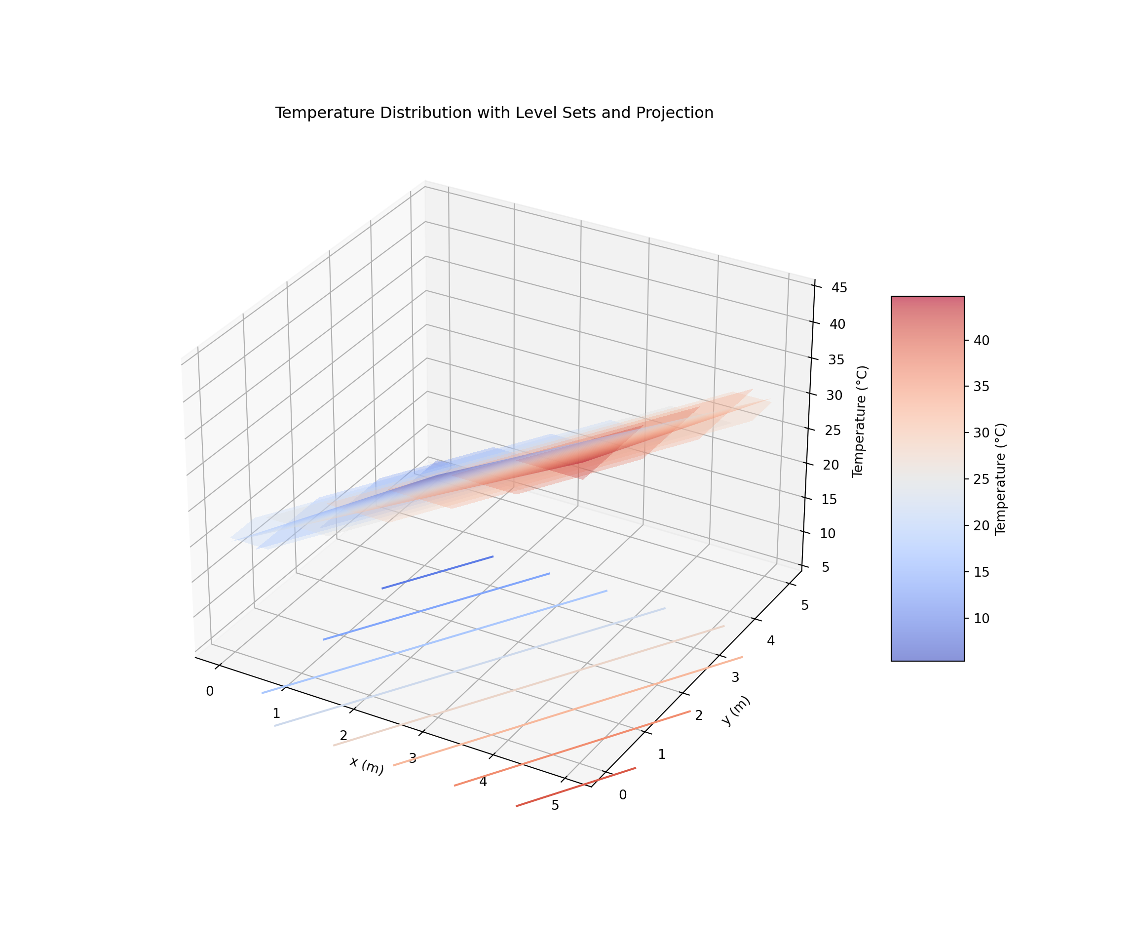

plt.show()

Example 2: Convex Function Visualization

Consider the function \(z = x^2 + y^2\), which is a classic example of a convex function in two variables. This function describes a paraboloid that opens upwards. As you move away from the origin, the value of \(z\) increases, and the level sets, represented by concentric circles centered at the origin, reflect this increase. To visualize this, the 3D surface plot displays the convex shape of the paraboloid, showing how the function behaves in three dimensions. The level sets are overlaid on the surface plot as contours indicating constant values of \(z\), helping to visualize the curvature of the surface. Additionally, the projection onto the \(xy\)-plane is depicted through a filled contour plot, which illustrates how the function’s value changes over the plane, providing a clear view of its distribution. The combined plot of the surface, level sets, and projection highlights the convex nature of \(z = x^2 + y^2\) and offers a comprehensive understanding of the function’s behavior.

Visualization of graph, level sets and projections are shown in the following plot.

import numpy as np
import matplotlib.pyplot as plt
from mpl_toolkits.mplot3d import Axes3D

# Define the coordinates
x = np.linspace(-5, 5, 100)
y = np.linspace(-5, 5, 100)
X, Y = np.meshgrid(x, y)

# Define the function
Z = X**2 + Y**2

# Create the figure and axis object
fig = plt.figure(figsize=(12, 10))
ax = fig.add_subplot(111, projection='3d')

# Plot the function surface (Graph)
surface = ax.plot_surface(X, Y, Z, cmap='viridis', alpha=0.6, edgecolor='none')

# Plot level sets
contour = ax.contour(X, Y, Z, levels=np.linspace(np.min(Z), np.max(Z), 10), cmap='viridis', linestyles='solid', offset=np.min(Z) - 10)

# Add projection onto the xy-plane
ax.contourf(X, Y, Z, levels=np.linspace(np.min(Z), np.max(Z), 10), cmap='viridis', alpha=0.3)

## <matplotlib.contour.QuadContourSet object at 0x0000029F572DCF10>

# Adding labels and title
ax.set_xlabel('x')

## Text(0.5, 0, 'x')

ax.set_ylabel('y')

## Text(0.5, 0.5, 'y')

ax.set_zlabel('z')

## Text(0.5, 0, 'z')

ax.set_title('Surface Plot of $z = x^2 + y^2$ with Level Sets and Projection')

## Text(0.5, 0.92, 'Surface Plot of $z = x^2 + y^2$ with Level Sets and Projection')

# Add a color bar to show the z scale
fig.colorbar(surface, ax=ax, shrink=0.5, aspect=5, label='z')

## <matplotlib.colorbar.Colorbar object at 0x0000029F572DCBE0>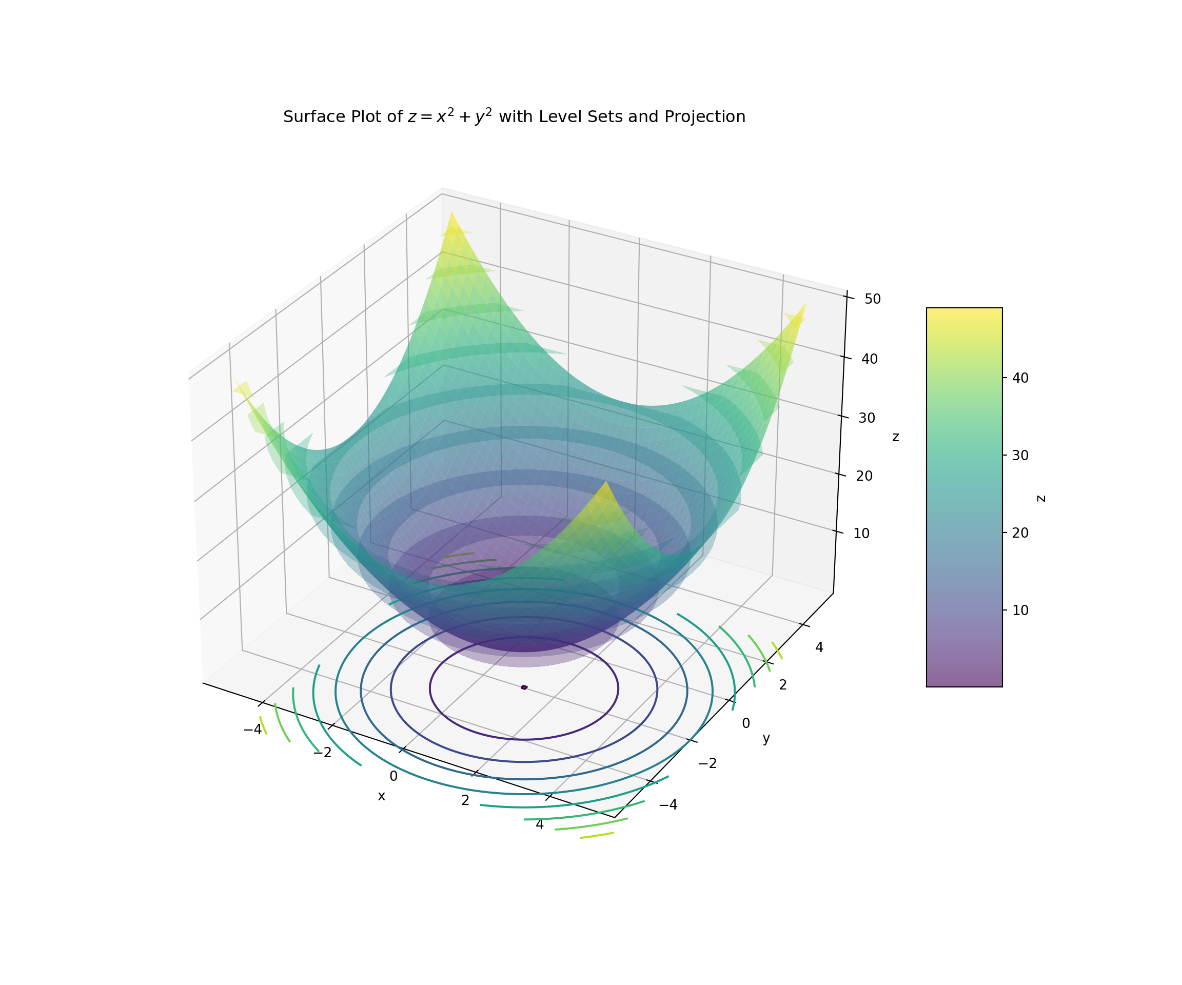

plt.show()

Example 3- Graph and Level sets of exponential function

Let’s consider a function \(f(x,y)=e^{-(x^2+y^2)}\). The contour lines of this function will be concentric circles with diminishing values as \(x^2+y^2\) increases. The complete behavious of this function is visualized as below:

import numpy as np
import matplotlib.pyplot as plt
from mpl_toolkits.mplot3d import Axes3D

# Define the coordinates
x = np.linspace(-3, 3, 100)
y = np.linspace(-3, 3, 100)
X, Y = np.meshgrid(x, y)

# Define the function
Z = np.exp(-(X**2 + Y**2))

# Create the figure
fig = plt.figure(figsize=(14, 10))
ax = fig.add_subplot(111, projection='3d')

# Plot the surface
surface = ax.plot_surface(X, Y, Z, cmap='viridis', alpha=0.7)

# Plot the contours
contours = ax.contour(X, Y, Z, levels=np.linspace(0, 1, 10), cmap='viridis', offset=0.1)
ax.clabel(contours, inline=True, fontsize=8)

# Adding labels and title
ax.set_xlabel('X axis')

## Text(0.5, 0, 'X axis')

ax.set_ylabel('Y axis')

## Text(0.5, 0.5, 'Y axis')

ax.set_zlabel('f(x, y)')

## Text(0.5, 0, 'f(x, y)')

ax.set_title('Graph and Level Sets of $f(x, y) = e^{-(x^2 + y^2)}$')

## Text(0.5, 0.92, 'Graph and Level Sets of $f(x, y) = e^{-(x^2 + y^2)}$')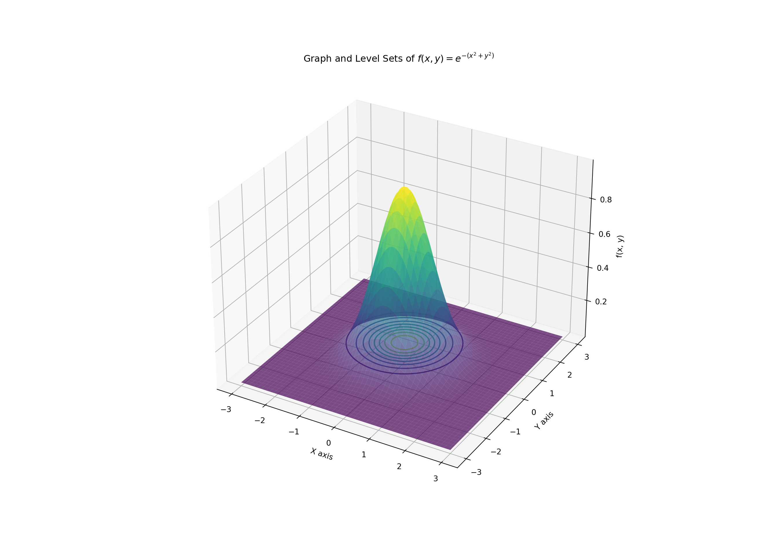

# Show the plot
plt.show()

### ### Limits for Functions of Two Variables

In multivariable calculus, the concept of limits for functions of two variables extends the idea from single-variable calculus. For a function \(f(x, y)\) of two variables, the limit as \((x, y)\) approaches a point \((a, b)\) is defined similarly: we seek to determine the value that \(f(x, y)\) approaches as the point \((x, y)\) gets arbitrarily close to \((a, b)\). Formally, the limit \(\lim_{(x, y) \to (a, b)} f(x, y)\) exists if, for every path approaching \((a, b)\) from any direction, the function values approach the same number.

The concept can be visualized by considering how \(f(x, y)\) behaves as \((x, y)\) gets close to \((a, b)\) from various paths. For instance, if we approach \((a, b)\) along a straight line, a curve, or any other path, the function should tend to the same value for the limit to exist. This helps in understanding the function’s behavior in a neighborhood around \((a, b)\) and is crucial for analyzing continuity and differentiability in higher dimensions.

Example of Limits for Functions of Two Variables

To illustrate the concept of limits for functions of two variables, consider the function \(f(x, y) = \frac{x^2 y}{x^2 + y^2}\) and evaluate the limit as \((x, y)\) approaches \((0, 0)\).

Example 1:

Let’s compute the limit of \(f(x, y) =\begin{cases} \frac{x^2 y}{x^2 + y^2};&\quad (x,y)\neq (0,0)\\0;&(x,y)=(0,0)\end{cases}\) as \((x, y) \to (0, 0)\).

Approach 1: Along the x-axis (\(y = 0\))

When \(y = 0\), \[ f(x, 0) = \frac{x^2 \cdot 0}{x^2 + 0^2} = 0 \]

Thus, as \(x \to 0\), \[ \lim_{x \to 0} f(x, 0) = 0 \]

Approach 2: Along the y-axis (\(x = 0\))

When \(x = 0\), \[ f(0, y) = \frac{0^2 \cdot y}{0^2 + y^2} = 0 \]

Thus, as \(y \to 0\), \[ \lim_{y \to 0} f(0, y) = 0 \]

Approach 3: Along the line \(y = x\)

When \(y = x\), \[ f(x, x) = \frac{x^2 \cdot x}{x^2 + x^2} = \frac{x^3}{2x^2} = \frac{x}{2} \]

Thus, as \(x \to 0\), \[ \lim_{x \to 0} f(x, x) = \frac{0}{2} = 0 \]

Since the limit is the same regardless of the path taken (x-axis, y-axis, or \(y = x\)), we conclude that: \[ \lim_{(x, y) \to (0, 0)} f(x, y) = 0 \]

Visualization

To visualize this, we will plot the function \(f(x, y)\) and show how the function behaves as \((x, y)\) approaches \((0, 0)\) from different paths.

import numpy as np
import matplotlib.pyplot as plt
from mpl_toolkits.mplot3d import Axes3D

# Define the coordinates
x = np.linspace(-2, 2, 100)
y = np.linspace(-2, 2, 100)
X, Y = np.meshgrid(x, y)

# Define the function
Z = np.where(X**2 + Y**2 != 0, (X**2 * Y) / (X**2 + Y**2), 0)  # Avoid division by zero

# Create the figure
fig = plt.figure(figsize=(14, 10))
ax = fig.add_subplot(111, projection='3d')

# Plot the surface
surface = ax.plot_surface(X, Y, Z, cmap='viridis', alpha=0.7, edgecolor='none')

# Plot the contours
contours = ax.contour(X, Y, Z, levels=np.linspace(-1, 1, 10), cmap='viridis', offset=np.min(Z))

# Adding labels and title
ax.set_xlabel('X axis')

## Text(0.5, 0, 'X axis')

ax.set_ylabel('Y axis')

## Text(0.5, 0.5, 'Y axis')

ax.set_zlabel('f(x, y)')

## Text(0.5, 0, 'f(x, y)')

ax.set_title('Graph and Contours of $f(x, y) = \\frac{x^2 y}{x^2 + y^2}$')

## Text(0.5, 0.92, 'Graph and Contours of $f(x, y) = \\frac{x^2 y}{x^2 + y^2}$')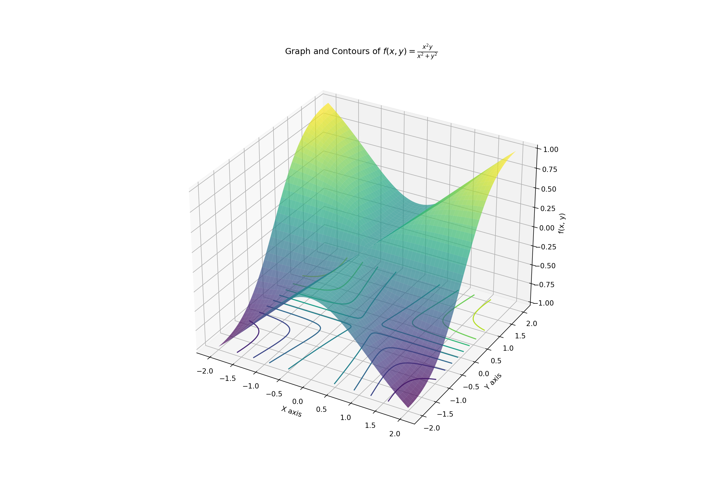

# Show the plot
plt.show()

Example 2: To illustrate the concept of limits for functions of two variables, consider the function \(f(x, y) = \frac{xy}{x^2 + y^2}\) and evaluate the limit as \((x, y)\) approaches \((0, 0)\).

Let’s compute the limit of \(f(x, y) = \frac{xy}{x^2 + y^2}\) as \((x, y) \to (0, 0)\).

Approach 1: Along the x-axis (\(y = 0\))

When \(y = 0\), \[ f(x, 0) = \frac{x \cdot 0}{x^2 + 0^2} = 0 \]

Thus, as \(x \to 0\), \[ \lim_{x \to 0} f(x, 0) = 0 \]

Approach 2: Along the y-axis (\(x = 0\))

When \(x = 0\), \[ f(0, y) = \frac{0 \cdot y}{0^2 + y^2} = 0 \]

Thus, as \(y \to 0\), \[ \lim_{y \to 0} f(0, y) = 0 \]

Approach 3: Along the line \(y = x\)

When \(y = x\), \[ f(x, x) = \frac{x \cdot x}{x^2 + x^2} = \frac{x^2}{2x^2} = \frac{1}{2} \]

Thus, as \(x \to 0\), \[ \lim_{x \to 0} f(x, x) = \frac{1}{2} \]

Since the limit along the line \(y = x\) is different from the limit along the x-axis and y-axis, we conclude that: \[ \lim_{(x, y) \to (0, 0)} f(x, y) \text{ does not exist.} \]

Visualization

To visualize this, we will plot the function \(f(x, y)\) and show how the function behaves as \((x, y)\) approaches \((0, 0)\) from different paths.

import numpy as np
import matplotlib.pyplot as plt
from mpl_toolkits.mplot3d import Axes3D

# Define the coordinates
x = np.linspace(-2, 2, 100)
y = np.linspace(-2, 2, 100)
X, Y = np.meshgrid(x, y)

# Define the function
Z = np.where(X**2 + Y**2 != 0, (X * Y) / (X**2 + Y**2), 0)  # Avoid division by zero

# Create the figure
fig = plt.figure(figsize=(14, 10))
ax = fig.add_subplot(111, projection='3d')

# Plot the surface
surface = ax.plot_surface(X, Y, Z, cmap='viridis', alpha=0.7, edgecolor='none')

# Plot the contours
contours = ax.contour(X, Y, Z, levels=np.linspace(-0.5, 0.5, 10), cmap='viridis', offset=np.min(Z))

# Adding labels and title
ax.set_xlabel('X axis')

## Text(0.5, 0, 'X axis')

ax.set_ylabel('Y axis')

## Text(0.5, 0.5, 'Y axis')

ax.set_zlabel('f(x, y)')

## Text(0.5, 0, 'f(x, y)')

ax.set_title('Graph and Contours of $f(x, y) = \\frac{xy}{x^2 + y^2}$')

## Text(0.5, 0.92, 'Graph and Contours of $f(x, y) = \\frac{xy}{x^2 + y^2}$')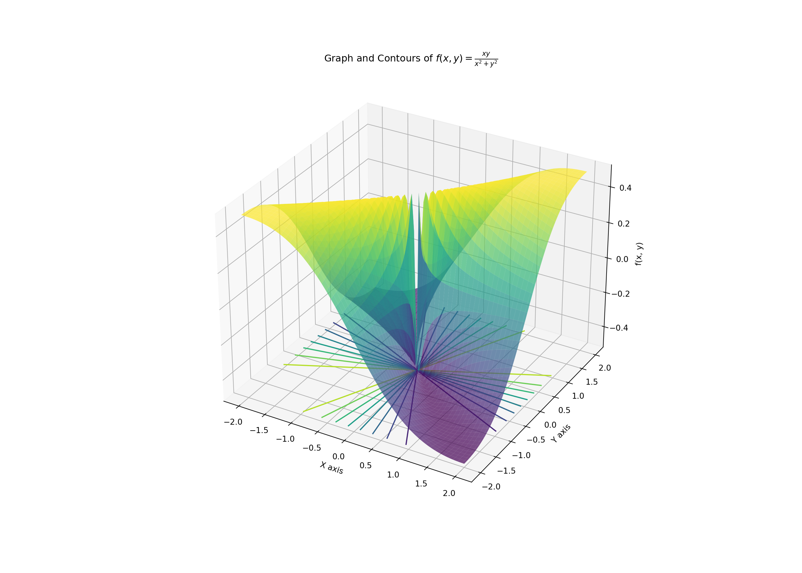

# Show the plot
plt.show()

Explanation using graph and contours:

• Graph: The 3D surface plot illustrates how \(f(x, y)\) varies in space. The function \(f(x, y) = \frac{xy}{x^2 + y^2}\) does not approach a single value as \((x, y)\) approaches \((0, 0)\). The surface shows different values depending on the path taken towards the origin. For example, along the x-axis and y-axis, the function tends to zero, while along the line \(y = x\), it tends to \(\frac{1}{2}\). This discrepancy in values along different paths confirms that the function does not have a single limit at the origin.

• Contours: The contour lines represent level sets of \(f(x, y)\). These lines show the function’s values across the \(xy\)-plane. The contour plot reveals varying values near the origin, indicating that the function behaves differently based on the direction from which \((x, y)\) approaches \((0, 0)\). The presence of multiple contours around the origin confirms that the limit of the function does not converge to a single value at that point.

By visualizing the function and its contours, we gain a clearer understanding of how \(f(x, y)\) behaves near the origin. The different values obtained from various paths of approach emphasize that the limit does not exist at \((0, 0)\).

3.7.4 Definition of Limit of a Bivariate Function

Let \(f(x, y)\) be a function defined on a domain in \(\mathbb{R}^2\), and let \((x_0, y_0)\) be a point in \(\mathbb{R}^2\). We say that the limit of \(f(x, y)\) as \((x, y)\) approaches \((x_0, y_0)\) exists and equals \(L\) if, for every \(\epsilon > 0\), there exists a \(\delta > 0\) such that for all \((x, y)\) in the domain, if \(0 < \sqrt{(x - x_0)^2 + (y - y_0)^2} < \delta\), then \(|f(x, y) - L| < \epsilon\). In mathematical notation:

\[ \lim_{(x, y) \to (x_0, y_0)} f(x, y) = L \]

if

\[ \forall \epsilon > 0, \; \exists \delta > 0 \text{ such that } \sqrt{(x - x_0)^2 + (y - y_0)^2} < \delta \implies |f(x, y) - L| < \epsilon. \]

Intuitive Definition: Intuitively, the limit of a bivariate function \(f(x, y)\) as \((x, y)\) approaches \((x_0, y_0)\) exists and equals \(L\) if, regardless of the path taken to approach \((x_0, y_0)\), the function \(f(x, y)\) approaches the same value \(L\). In other words, the value of \(f(x, y)\) converges to \(L\) uniquely, irrespective of the direction or path along which \((x, y)\) approaches \((x_0, y_0)\).

Example with Intuition

Consider the function \(f(x, y) = \frac{xy}{x^2 + y^2}\). If we approach \((0, 0)\) along the x-axis (\(y = 0\)), the function value approaches 0. If we approach along the y-axis (\(x = 0\)), the function value also approaches 0. However, if we approach along the line \(y = x\), the function value approaches \(\frac{1}{2}\). Since the function approaches different values depending on the path taken, the limit does not exist at \((0, 0)\). For a limit to exist, \(f(x, y)\) must approach the same value regardless of the path.

Example- Application of Limit in Digital Image Processing:

In image processing, the concept of limits for functions of two variables is crucial for operations such as edge detection. Let’s consider a simple example involving the gradient of an image. Suppose we have a grayscale image where each pixel intensity is a function of its position \((x, y)\). For instance, the image intensity function \(f(x, y)\) might be modeled by:

\[ f(x, y) = e^{-(x^2 + y^2)} \]

This function represents a Gaussian distribution centered at the origin. We want to analyze how the intensity of the image changes as we move away from the center, which can help in detecting edges.

To visualize this, we can plot the Gaussian function \(f(x, y) = e^{-(x^2 + y^2)}\) and its level sets to understand how the intensity changes.

Here’s the code to visualize the function, its level sets, and its gradient:

import numpy as np
import matplotlib.pyplot as plt
from mpl_toolkits.mplot3d import Axes3D

# Define the function
def f(x, y):
    return np.exp(-(x**2 + y**2))

# Create a grid of x, y values
x = np.linspace(-2, 2, 100)
y = np.linspace(-2, 2, 100)
X, Y = np.meshgrid(x, y)
Z = f(X, Y)

# Create figure
fig = plt.figure(figsize=(12, 6))

# Plot the surface
ax1 = fig.add_subplot(121, projection='3d')
ax1.plot_surface(X, Y, Z, cmap='viridis', edgecolor='none')

## <mpl_toolkits.mplot3d.art3d.Poly3DCollection object at 0x0000029F596AFD00>

ax1.set_title('3D Surface Plot of $f(x, y) = e^{-(x^2 + y^2)}$')

## Text(0.5, 0.92, '3D Surface Plot of $f(x, y) = e^{-(x^2 + y^2)}$')

ax1.set_xlabel('x')

## Text(0.5, 0, 'x')

ax1.set_ylabel('y')

## Text(0.5, 0.5, 'y')

ax1.set_zlabel('f(x, y)')

## Text(0.5, 0, 'f(x, y)')

# Plot the contour
ax2 = fig.add_subplot(122)
contour = ax2.contour(X, Y, Z, levels=10, cmap='viridis')
ax2.set_title('Contour Plot of $f(x, y) = e^{-(x^2 + y^2)}$')

## Text(0.5, 1.0, 'Contour Plot of $f(x, y) = e^{-(x^2 + y^2)}$')

ax2.set_xlabel('x')

## Text(0.5, 0, 'x')

ax2.set_ylabel('y')

## Text(0, 0.5, 'y')

# Show plot
plt.colorbar(contour, ax=ax2)

## <matplotlib.colorbar.Colorbar object at 0x0000029F593ED280>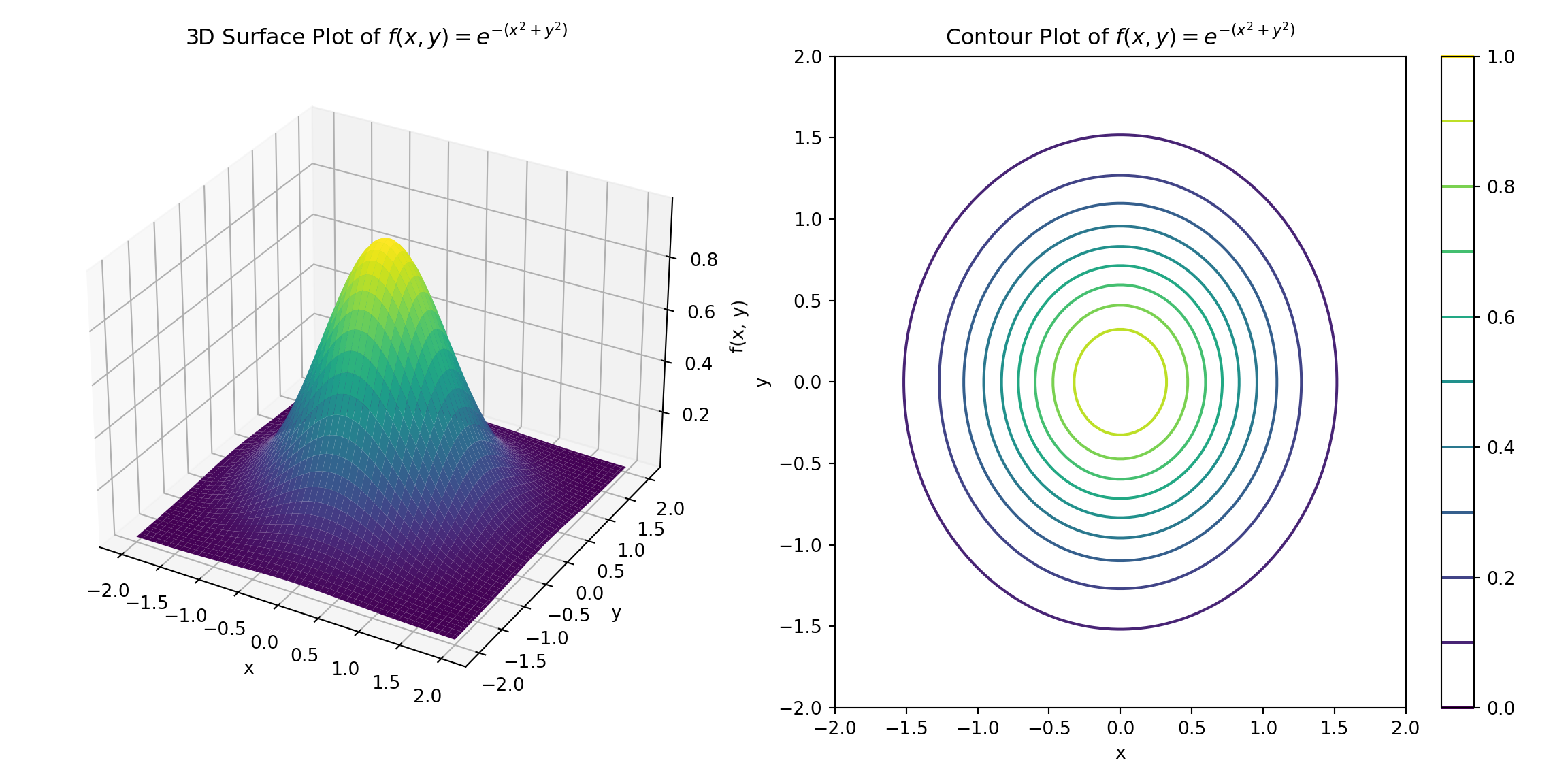

plt.tight_layout()
plt.show()

3.7.4.1 Explanation

1. Surface Plot: The 3D surface plot illustrates how the intensity \(f(x, y)\) decreases as we move away from the center (origin). This provides a visual representation of how intensity values vary with position. In this plot, you can observe how the intensity diminishes from the center outward.

2. Contour Plot: The contour plot displays level sets of the function \(f(x, y)\). Each contour represents a constant intensity level, showing where the intensity remains the same. This is useful for edge detection as the contours highlight boundaries between different regions with varying intensities.

This example shows how understanding the limits and behavior of functions of two variables is applied in real-world computer science problems, particularly in image processing and machine learning tasks.

3.7.4.2 Practice Problems:

---

Problem 1:
Find the limit of \(f(x, y) = \frac{x^2 + y^2}{x^2 + y^2}\) as \((x, y) \to (0, 0)\).

Solution:
For \((x, y) \neq (0, 0)\), we have: \[ f(x, y) = \frac{x^2 + y^2}{x^2 + y^2} = 1 \] The limit as \((x, y) \to (0, 0)\) is simply 1.

---

Problem 2:
Determine whether the limit of \(f(x, y) = \frac{xy}{x^2 + y^2}\) exists as \((x, y) \to (0, 0)\) and find it if it does.

Solution:
Approach along \(y = x\): \[ f(x, x) = \frac{x^2}{x^2 + x^2} = \frac{1}{2} \]

Approach along \(y = -x\): \[ f(x, -x) = \frac{-x^2}{x^2 + x^2} = -\frac{1}{2} \]

Since the limit depends on the path, it does not exist.

---

Problem 3:
Find the limit of \(f(x, y) = \frac{3x^2 + 4y^2}{2x^2 + y^2}\) as \((x, y) \to (0, 0)\).

Solution:
\[ f(x, y) = \frac{3x^2 + 4y^2}{2x^2 + y^2} \] For \((x, y) \neq (0, 0)\), this function simplifies to: \[ \frac{3x^2 + 4y^2}{2x^2 + y^2} \] As \((x, y) \to (0, 0)\), the numerator and denominator both approach 0, but their ratio approaches: \[ \frac{0}{0} \] To investigate further, we use polar coordinates \(x = r \cos(\theta)\) and \(y = r \sin(\theta)\): \[ f(r, \theta) = \frac{3r^2 \cos^2(\theta) + 4r^2 \sin^2(\theta)}{2r^2 \cos^2(\theta) + r^2 \sin^2(\theta)} = \frac{3 \cos^2(\theta) + 4 \sin^2(\theta)}{2 \cos^2(\theta) + \sin^2(\theta)} \] The limit exists and is given by the above expression.

---

Problem 4:
Determine whether the limit of \(f(x, y) = \frac{x^3 + y^3}{x^2 + y^2}\) exists as \((x, y) \to (0, 0)\) and find it if it does.

Solution:
Approach along \(y = 0\): \[ f(x, 0) = \frac{x^3}{x^2} = x \] As \(x \to 0\), \(f(x, 0) \to 0\).

Approach along \(x = 0\): \[ f(0, y) = \frac{y^3}{y^2} = y \] As \(y \to 0\), \(f(0, y) \to 0\).

The limit exists and is 0.

---

Problem 5:
Find the limit of \(f(x, y) = \sin\left(\frac{x}{y}\right)\) as \((x, y) \to (0, 0)\).

Solution:
For \((x, y) \neq (0, 0)\), the function \(\sin\left(\frac{x}{y}\right)\) oscillates infinitely as \((x, y) \to (0, 0)\). Thus, the limit does not exist.

---

Problem 6:
Determine the limit of \(f(x, y) = \frac{e^{x+y} - e^x}{y}\) as \((x, y) \to (0, 0)\).

Solution:
Use L’Hôpital’s rule with respect to \(y\): \[ \lim_{y \to 0} \frac{e^{x+y} - e^x}{y} = \lim_{y \to 0} \frac{e^{x+y}}{1} = e^x \] As \((x, y) \to (0, 0)\), the limit is \(e^0 = 1\).

---

Problem 7:
Find the limit of \(f(x, y) = \frac{x^2 - y^2}{x^2 + y^2}\) as \((x, y) \to (0, 0)\).

Solution:
Approach along \(y = x\): \[ f(x, x) = \frac{x^2 - x^2}{x^2 + x^2} = 0 \]

Approach along \(y = -x\): \[ f(x, -x) = \frac{x^2 - x^2}{x^2 + x^2} = 0 \]

The limit exists and is 0.

---

Problem 8:
Determine whether the limit of \(f(x, y) = \frac{x^2 + xy + y^2}{x^2 - xy + y^2}\) exists as \((x, y) \to (0, 0)\) and find it if it does.

Solution:
Use polar coordinates: \[ f(r, \theta) = \frac{r^2 (\cos^2(\theta) + \cos(\theta) \sin(\theta) + \sin^2(\theta))}{r^2 (\cos^2(\theta) - \cos(\theta) \sin(\theta) + \sin^2(\theta))} = \frac{1 + \cos(\theta) \sin(\theta)}{1 - \cos(\theta) \sin(\theta)} \] The limit exists and is given by the above expression.

---

Problem 9:
Find the limit of \(f(x, y) = \frac{\sqrt{x^2 + y^2}}{x^2 + y^2}\) as \((x, y) \to (0, 0)\).

Solution:
Use polar coordinates: \[ f(r, \theta) = \frac{r}{r^2} = \frac{1}{r} \] As \(r \to 0\), \(\frac{1}{r} \to \infty\). Thus, the limit does not exist.

---

Problem 10:
Determine whether the limit of \(f(x, y) = \frac{x^3 - 3xy^2}{x^2 + y^2}\) exists as \((x, y) \to (0, 0)\) and find it if it does.

Solution:
Use polar coordinates: \[ f(r, \theta) = \frac{r^3 (\cos^3(\theta) - 3 \cos(\theta) \sin^2(\theta))}{r^2} = r (\cos^3(\theta) - 3 \cos(\theta) \sin^2(\theta)) \] As \(r \to 0\), \(f(r, \theta) \to 0\). The limit exists and is 0.

---

Call-Out Note: Proving Non-Existence of Limits

To prove that the limit of a function \(f(x, y)\) as \((x, y) \to (x_0, y_0)\) does not exist, it is often sufficient to find just one path along which the limit differs from the limit along another path, or where the limit depends on a parameter. This method demonstrates that the limit varies based on the approach to the point.

Here are some examples to illustrate this concept:

1. Example 1:

   Consider \(f(x, y) = \frac{xy}{x^2 + y^2}\). We will check the limit along different paths:

   • Along the path \(y = mx\) (where \(m\) is a constant): \[ f(x, mx) = \frac{x(mx)}{x^2 + (mx)^2} = \frac{mx^2}{x^2 + m^2x^2} = \frac{mx^2}{x^2(1 + m^2)} = \frac{m}{1 + m^2} \] As \((x, y) \to (0, 0)\), this approaches \(\frac{m}{1 + m^2}\), which depends on the value of \(m\).

   Since the limit depends on \(m\), the limit does not exist as it varies with different values of \(m\).

2. Example 2:

   For \(f(x, y) = \frac{e^x - e^y}{x - y}\), consider:

   • Along the path \(y = 0\): \[ f(x, 0) = \frac{e^x - e^0}{x - 0} = \frac{e^x - 1}{x} \] As \(x \to 0\), this approaches \(1\) (using L’Hôpital’s Rule).
   • Along the path \(y = x/2\): \[ f(x, x/2) = \frac{e^x - e^{x/2}}{x - x/2} = \frac{e^x - e^{x/2}}{x/2} = \frac{2(e^x - e^{x/2})}{x} \] As \(x \to 0\), this approaches a different value depending on the rates of change of \(e^x\) and \(e^{x/2}\).

   The varying limits along different paths indicate the limit does not exist.

3. Example 3:

   Consider \(f(x, y) = \frac{xy}{x^2 + y^2}\). Check the limit along various paths:

   • Along the path \(y = mx\) (where \(m\) is a constant): \[ f(x, mx) = \frac{x(mx)}{x^2 + (mx)^2} = \frac{mx^2}{x^2 + m^2x^2} = \frac{mx^2}{x^2(1 + m^2)} = \frac{m}{1 + m^2} \] As \((x, y) \to (0, 0)\), this approaches \(\frac{m}{1 + m^2}\), which varies with different values of \(m\).

   • Along the path \(y = x^2\): \[ f(x, x^2) = \frac{x \cdot x^2}{x^2 + (x^2)^2} = \frac{x^3}{x^2 + x^4} = \frac{x^3}{x^2(1 + x^2)} = \frac{x}{1 + x^2} \] As \(x \to 0\), this approaches \(0\).

   The limit depends on the path taken. Along \(y = mx\), it depends on \(m\), while along \(y = x^2\), it approaches \(0\). Hence, the limit does not exist.

By choosing various paths, you can demonstrate that the limit varies or depends on the approach, thereby proving that the limit does not exist.

3.7.5 Extending Continuity from Single-Variable to Bivariate Functions

In Module 1, we explored the concept of continuity for single-variable functions. Recall that a function \(f(x)\) is continuous at a point \(x = a\) if:

1. The function value \(f(a)\) is defined.
2. The limit of \(f(x)\) as \(x\) approaches \(a\) exists.
3. This limit is equal to the function value \(f(a)\).

In extending this concept to functions of two variables, \(f(x, y)\), we apply a similar set of conditions but in a higher-dimensional space.

Continuity for Bivariate Functions

For a function \(f(x, y)\) of two variables, we say that \(f(x, y)\) is continuous at a point \((x_0, y_0)\) if:

1. Defined: The function \(f(x, y)\) is defined at \((x_0, y_0)\).
2. Limit Exists: The limit of \(f(x, y)\) as \((x, y)\) approaches \((x_0, y_0)\) exists.
3. Limit Equals Function Value: The limit of \(f(x, y)\) as \((x, y)\) approaches \((x_0, y_0)\) is equal to \(f(x_0, y_0)\).

Mathematically, this is expressed as: \[ \text{The function } f(x, y) \text{ is continuous at } (x_0, y_0) \text{ if:} \] \[ \lim_{(x, y) \to (x_0, y_0)} f(x, y) = f(x_0, y_0). \]

Intuitive Understanding: To understand this in a practical context, think of a function \(f(x, y)\) as a surface in three-dimensional space. For the function to be continuous at a point \((x_0, y_0)\), you should be able to draw the surface around that point without any jumps or breaks. The value of the function at \((x_0, y_0)\) should match the value that you approach from any direction.

Example:

Consider the function \(f(x, y) = x^2 + y^2\). To determine its continuity at a point \((a, b)\):

1. Defined: The function \(f(a, b) = a^2 + b^2\) is clearly defined for any point \((a, b)\).
2. Limit Exists: As \((x, y) \to (a, b)\), the limit of \(f(x, y)\) is: \[ \lim_{(x, y) \to (a, b)} (x^2 + y^2) = a^2 + b^2. \]
3. Limit Equals Function Value: Since \(f(a, b) = a^2 + b^2\), the limit equals the function value.

Thus, \(f(x, y) = x^2 + y^2\) is continuous at all points \((a, b)\). This demonstrates the seamless transition from single-variable to bivariate functions, where continuity maintains its core principle of no abrupt changes or discontinuities.

3.7.5.1 Problems and Solutions on Checking Continuity at a Point

1. Problem 1: Determine if the function \(f(x, y) = \frac{x^2 - y^2}{x^2 + y^2}\) is continuous at \((0, 0)\).

   Solution:

   • The function is not defined at \((0, 0)\) since the denominator becomes zero.
   • Along the path \(y = x\), \(f(x, x) = \frac{x^2 - x^2}{x^2 + x^2} = 0\).
   • Along the path \(y = -x\), \(f(x, -x) = \frac{x^2 - (-x)^2}{x^2 + (-x)^2} = 0\).
   • The limit as \((x, y) \to (0, 0)\) is not well-defined because the function is not defined at \((0, 0)\). Therefore, \(f\) is not continuous at \((0, 0)\).

2. Problem 2: Check if \(f(x, y) = \frac{xy}{x^2 + y^2}\) is continuous at \((0, 0)\).

   Solution:

   • The function is not defined at \((0, 0)\) since the denominator becomes zero.
   • Along the path \(y = x\), \(f(x, x) = \frac{x \cdot x}{x^2 + x^2} = \frac{x^2}{2x^2} = \frac{1}{2}\).
   • Along the path \(y = -x\), \(f(x, -x) = \frac{x \cdot (-x)}{x^2 + (-x)^2} = \frac{-x^2}{2x^2} = -\frac{1}{2}\).
   • The limit depends on the path taken. Therefore, \(f\) is not continuous at \((0, 0)\).

3. Problem 3: Determine if \(f(x, y) = \frac{2x^3 - 3xy^2}{x^2 + y^2}\) is continuous at \((0, 0)\).

   Solution:

   • The function is not defined at \((0, 0)\) since the denominator becomes zero.
   • Along the path \(y = 0\), \(f(x, 0) = \frac{2x^3 - 0}{x^2 + 0} = \frac{2x^3}{x^2} = 2x\), which tends to \(0\) as \(x \to 0\).
   • Along the path \(x = 0\), \(f(0, y) = \frac{0 - 3 \cdot 0}{0 + y^2} = 0\), which is \(0\).
   • Along the path \(y = kx\), \(f(x, kx) = \frac{2x^3 - 3x(kx)^2}{x^2 + (kx)^2} = \frac{2x^3 - 3k^2x^3}{x^2 + k^2x^2} = \frac{2 - 3k^2}{1 + k^2} x\), which tends to \(0\) as \(x \to 0\).
   • The limit is \(0\) along all paths. Therefore, \(f\) is continuous at \((0, 0)\).

4. Problem 4: Check the continuity of \(f(x, y) = \frac{x^2 + y^2}{x^2 - y^2}\) at \((1, 1)\).

   Solution:

   • Substituting \(x = 1\) and \(y = 1\) into the function: \(f(1, 1) = \frac{1^2 + 1^2}{1^2 - 1^2} = \frac{2}{0}\).
   • The function is undefined at \((1, 1)\). Therefore, \(f\) is not continuous at \((1, 1)\).

5. Problem 5: Determine if \(f(x, y) = e^{-(x^2 + y^2)}\) is continuous at \((0, 0)\).

   Solution:

   • The function \(f(x, y) = e^{-(x^2 + y^2)}\) is defined for all \((x, y)\).
   • Substituting \((0, 0)\), \(f(0, 0) = e^{-(0^2 + 0^2)} = e^0 = 1\).
   • For any \((x, y)\), \(f(x, y)\) is continuous because the exponential function is continuous and the argument \(-(x^2 + y^2)\) is continuous.
   • Therefore, \(f\) is continuous at \((0, 0)\).

6. Problem 6: Determine the continuity of \(f(x, y) = \frac{x^2 - y^2}{x - y}\) at \((0, 0)\).

   Solution:

   • The function is not defined at \((0, 0)\) since the denominator becomes zero.
   • Rewrite \(\frac{x^2 - y^2}{x - y} = x + y\) when \(x \neq y\).
   • Along the path \(x = y\), the function simplifies to \(\frac{x^2 - x^2}{x - x} = \text{undefined}\).
   • Along the path \(y = 0\), \(f(x, 0) = \frac{x^2 - 0}{x - 0} = x\), which tends to \(0\) as \(x \to 0\).
   • Along the path \(x = 0\), \(f(0, y) = \frac{0 - y^2}{0 - y} = y\), which tends to \(0\) as \(y \to 0\).
   • The limit depends on the path taken. Therefore, \(f\) is not continuous at \((0, 0)\).

7. Problem 7: Determine if \(f(x, y) = \frac{x^2 + y^2}{x^2 + 2y^2}\) is continuous at \((0, 0)\).

   Solution:

   • The function is not defined at \((0, 0)\) since the denominator becomes zero.
   • Along the path \(y = 0\), \(f(x, 0) = \frac{x^2}{x^2} = 1\).
   • Along the path \(x = 0\), \(f(0, y) = \frac{y^2}{2y^2} = \frac{1}{2}\).
   • The limit depends on the path taken. Therefore, \(f\) is not continuous at \((0, 0)\).

8. Problem 8: Check the continuity of \(f(x, y) = \frac{x^2 - 2xy + y^2}{x^2 + y^2}\) at \((1, 1)\).

   Solution:

   • Substituting \((1, 1)\), \(f(1, 1) = \frac{1^2 - 2 \cdot 1 \cdot 1 + 1^2}{1^2 + 1^2} = \frac{1 - 2 + 1}{2} = 0\).
   • The function is defined and continuous at \((1, 1)\).

9. Problem 9: Determine if \(f(x, y) = \frac{2x^2 - 3y^2}{x^2 + y^2}\) is continuous at \((0, 0)\).

   Solution:

   • The function is not defined at \((0, 0)\) since the denominator becomes zero.
   • Along the path \(y = 0\), \(f(x, 0) = \frac{2x^2}{x^2} = 2\).
   • Along the path \(x = 0\), \(f(0, y) = \frac{-3y^2}{y^2} = -3\).
   • The limit depends on the path taken. Therefore, \(f\) is not continuous at \((0, 0)\).

10. Problem 10: Determine if \(f(x, y) = \frac{x^3 - y^3}{x^2 + y^2}\) is continuous at \((0, 0)\).

    Solution:

    • The function is not defined at \((0, 0)\) since the denominator becomes zero.
    • Along the path \(y = 0\), \(f(x, 0) = \frac{x^3}{x^2} = x\), which tends to \(0\) as \(x \to 0\).
    • Along the path \(x = 0\), \(f(0, y) = \frac{-y^3}{y^2} = -y\), which tends to \(0\) as \(y \to 0\).
    • Along the path \(y = x\), \(f(x, x) = \frac{x^3 - x^3}{x^2 + x^2} = 0\).
    • The limit is \(0\) along all paths. Therefore, \(f\) is continuous at \((0, 0)\).

11. Problem 11: Check the continuity of \(f(x, y) = \frac{x^2 - y^2}{x - y}\) at \((0, 0)\).

    Solution:

    • Rewrite \(f(x, y) = \frac{x^2 - y^2}{x - y} = x + y\) for \(x \neq y\).
    • Along the path \(x = y\), the function is undefined.
    • Along the path \(y = 0\), \(f(x, 0) = x\), which tends to \(0\) as \(x \to 0\).
    • Along the path \(x = 0\), \(f(0, y) = -y\), which tends to \(0\) as \(y \to 0\).
    • The function simplifies to \(x + y\), which is continuous everywhere except along the line \(x = y\). Therefore, \(f\) is not continuous at \((0, 0)\).

3.7.6 Partial Derivatives

In multivariable calculus, partial derivatives extend the concept of derivatives to functions of more than one variable. For a function \(f(x, y)\), the partial derivative with respect to one variable measures how the function changes as that variable changes, while keeping the other variables constant. This concept is crucial in fields such as computer science, engineering, and data science where functions often depend on multiple parameters.

Reasoning Behind Partial Derivatives

Consider a bivariate function \(f(x, y)\). Unlike univariate functions where the rate of change is determined by a single variable, a bivariate function’s behavior depends on two variables. The partial derivatives help us understand how \(f\) changes in each direction separately:

1. Partial Derivative with Respect to \(x\) ( \(\frac{\partial f}{\partial x}\) ): This measures the rate of change of \(f\) as \(x\) changes while \(y\) is held constant. It answers the question: “How does the function \(f\) change if only the \(x\) component of the input changes?”

2. Partial Derivative with Respect to \(y\) ( \(\frac{\partial f}{\partial y}\) ): This measures the rate of change of \(f\) as \(y\) changes while \(x\) is held constant. It answers the question: “How does the function \(f\) change if only the \(y\) component of the input changes?”

Formal Definition of Partial Derivatives at a point

In multivariable calculus, partial derivatives are used to measure how a function of several variables changes as one variable changes, while the other variables are held constant.

Definition: Given a function \(f(x, y)\) of two variables \(x\) and \(y\), the partial derivative of \(f\) with respect to \(x\) at a point \((x_0, y_0)\) is defined as:

\[ \frac{\partial f}{\partial x}(x_0, y_0) = \lim_{h \to 0} \frac{f(x_0 + h, y_0) - f(x_0, y_0)}{h} \]

where \(h\) is a small increment in the \(x\)-direction.

Similarly, the partial derivative of \(f\) with respect to \(y\) at \((x_0, y_0)\) is:

\[ \frac{\partial f}{\partial y}(x_0, y_0) = \lim_{k \to 0} \frac{f(x_0, y_0 + k) - f(x_0, y_0)}{k} \]

where \(k\) is a small increment in the \(y\)-direction.

Interpretation

• Partial Derivative with Respect to \(x\): Measures the rate of change of the function \(f\) as \(x\) changes, while keeping \(y\) fixed.
• Partial Derivative with Respect to \(y\): Measures the rate of change of the function \(f\) as \(y\) changes, while keeping \(x\) fixed.

Example:

Consider the function \(f(x, y) = x^2 y + 3x y^2\). To find the partial derivatives:

1. Partial Derivative with Respect to \(x\) at \((1, 2)\): \[ \frac{\partial f}{\partial x}(1, 2) = \lim_{h \to 0} \frac{f(1 + h, 2) - f(1, 2)}{h} \]

   Calculate: \[ f(1 + h, 2) = (1 + h)^2 \cdot 2 + 3 \cdot (1 + h) \cdot 2^2 \] \[ f(1, 2) = 1^2 \cdot 2 + 3 \cdot 1 \cdot 2^2 = 2 + 12 = 14 \] \[ \frac{\partial f}{\partial x}(1, 2) = \lim_{h \to 0} \frac{(1 + h)^2 \cdot 2 + 3 \cdot (1 + h) \cdot 4 - 14}{h} \] \[ = \lim_{h \to 0} \frac{2 + 4h + h^2 \cdot 2 + 12 + 12h - 14}{h} \] \[ = \lim_{h \to 0} \frac{2h + 2h^2 + 12h}{h} = \lim_{h \to 0} \frac{14h + 2h^2}{h} = 14 \]

2. Partial Derivative with Respect to \(y\) at \((1, 2)\): \[ \frac{\partial f}{\partial y}(1, 2) = \lim_{k \to 0} \frac{f(1, 2 + k) - f(1, 2)}{k} \]

   Calculate: \[ f(1, 2 + k) = 1^2 \cdot (2 + k) + 3 \cdot 1 \cdot (2 + k)^2 \] \[ f(1, 2) = 14 \] \[ \frac{\partial f}{\partial y}(1, 2) = \lim_{k \to 0} \frac{1 \cdot (2 + k) + 3 \cdot (2 + k)^2 - 14}{k} \] \[ = \lim_{k \to 0} \frac{2 + k + 3 \cdot (4 + 4k + k^2) - 14}{k} \] \[ = \lim_{k \to 0} \frac{2 + k + 12 + 12k + 3k^2 - 14}{k} \] \[ = \lim_{k \to 0} \frac{12k + 3k^2}{k} = \lim_{k \to 0} (12 + 3k) = 12 \]

In this way, partial derivatives help us understand how the function behaves in each direction independently.

Following definition of derivatives alone:

Let’s consider the above function: \[ f(x, y) = x^2 y + 3xy^2 \]

To find the partial derivatives, follow these steps:

1. Partial Derivative with Respect to \(x\): \[ \frac{\partial f}{\partial x} = \frac{\partial}{\partial x} (x^2 y + 3xy^2) \] Here, treat \(y\) as a constant: \[ \frac{\partial f}{\partial x} = 2xy + 3y^2 \]

2. Partial Derivative with Respect to \(y\): \[ \frac{\partial f}{\partial y} = \frac{\partial}{\partial y} (x^2 y + 3xy^2) \] Here, treat \(x\) as a constant: \[ \frac{\partial f}{\partial y} = x^2 + 6xy \]

In practical scenarios, such as training machine learning models or designing systems, partial derivatives are used to analyze sensitivity to parameters and guide adjustments for improved performance.

Example: Illustrating Breakdance Movements with Partial Derivatives

In the context of breakdance movements on a sphere, we can visualize the movement and analyze it using partial derivatives. The partial derivatives can provide insights into how different parts of the body (hands, legs, and head) move relative to each other.

To visualize the movements and extract the partial derivatives, follow these steps:

1. Define the Movement Function

   Suppose we define the movement on the surface of a sphere using spherical coordinates \((r, \theta, \phi)\). For simplicity, let’s consider the following functions for different body parts:

   • Hands: Movement in the \(\theta\) direction.
   • Legs: Movement in the \(\phi\) direction.
   • Head: Combined effect of movements in both \(\theta\) and \(\phi\).

   The movement function can be represented as: \[ f(\theta, \phi) = \sin(\theta) \cdot \cos(\phi) \]

2. Compute Partial Derivatives

   • Partial Derivative with respect to \(\theta\): Represents how the movement changes with respect to the angle \(\theta\) (e.g., hand movement). \[ \frac{\partial f}{\partial \theta} = \cos(\theta) \cdot \cos(\phi) \]

   • Partial Derivative with respect to \(\phi\): Represents how the movement changes with respect to the angle \(\phi\) (e.g., leg movement). \[ \frac{\partial f}{\partial \phi} = -\sin(\theta) \cdot \sin(\phi) \]

Here’s a Python code snippet to visualize these movements and partial derivatives:

import numpy as np
import matplotlib.pyplot as plt
from mpl_toolkits.mplot3d import Axes3D

# Parameters
theta = np.linspace(0, np.pi, 100)
phi = np.linspace(0, 2 * np.pi, 100)
THETA, PHI = np.meshgrid(theta, phi)

# Movement function
R = np.sin(THETA) * np.cos(PHI)

# Compute partial derivatives
dR_dtheta = np.cos(THETA) * np.cos(PHI)
dR_dphi = -np.sin(THETA) * np.sin(PHI)

# Create 3D plot
fig = plt.figure(figsize=(14, 8))
ax = fig.add_subplot(111, projection='3d')

# Plot movement function
ax.plot_surface(R * np.sin(THETA) * np.cos(PHI), 
                 R * np.sin(THETA) * np.sin(PHI), 
                 R * np.cos(THETA), 
                 cmap='viridis', alpha=0.5)

## <mpl_toolkits.mplot3d.art3d.Poly3DCollection object at 0x0000029F58F08D60>

# Plot partial derivatives
ax.quiver(R * np.sin(THETA) * np.cos(PHI), 
          R * np.sin(THETA) * np.sin(PHI), 
          R * np.cos(THETA), 
          dR_dtheta, 
          dR_dphi, 
          np.zeros_like(dR_dtheta), 
          length=0.1, normalize=True, color='blue', label='Partial Derivative w.r.t. theta')

## <mpl_toolkits.mplot3d.art3d.Line3DCollection object at 0x0000029F58F10040>

ax.quiver(R * np.sin(THETA) * np.cos(PHI), 
          R * np.sin(THETA) * np.sin(PHI), 
          R * np.cos(THETA), 
          np.zeros_like(dR_dphi), 
          np.zeros_like(dR_dphi), 
          dR_dphi, 
          length=0.1, normalize=True, color='red', label='Partial Derivative w.r.t. phi')

## <mpl_toolkits.mplot3d.art3d.Line3DCollection object at 0x0000029F58F089A0>

# Labels and title
ax.set_xlabel('X-axis')

## Text(0.5, 0, 'X-axis')

ax.set_ylabel('Y-axis')

## Text(0.5, 0.5, 'Y-axis')

ax.set_zlabel('Z-axis')

## Text(0.5, 0, 'Z-axis')

ax.set_title('Breakdance Movements with Partial Derivatives')

## Text(0.5, 0.92, 'Breakdance Movements with Partial Derivatives')

ax.legend()

## <matplotlib.legend.Legend object at 0x0000029F58CCA3D0>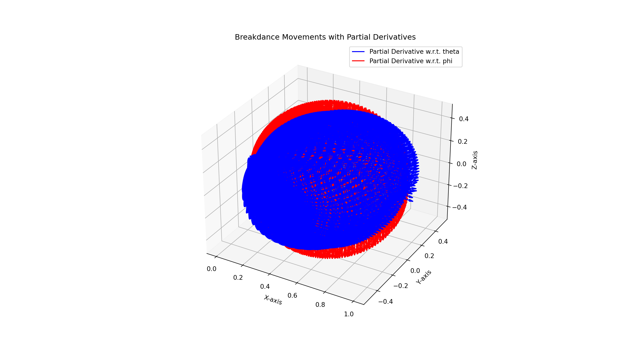

plt.show()

3.7.6.1 Partial Derivatives Problems

1. Find the partial derivatives of \(f(x, y) = 3x^2 y + 5xy^2\) with respect to \(x\) and \(y\).

   Solution: \[ \frac{\partial f}{\partial x} = 6xy + 5y^2 \] \[ \frac{\partial f}{\partial y} = 3x^2 + 10xy \]

2. Find the partial derivatives of \(f(x, y) = e^{x+y}\) with respect to \(x\) and \(y\).

   Solution: \[ \frac{\partial f}{\partial x} = e^{x+y} \] \[ \frac{\partial f}{\partial y} = e^{x+y} \]

3. Find the partial derivatives of \(f(x, y) = \sin(xy)\) with respect to \(x\) and \(y\).

   Solution: \[ \frac{\partial f}{\partial x} = y \cos(xy) \] \[ \frac{\partial f}{\partial y} = x \cos(xy) \]

4. Find the partial derivatives of \(f(x, y) = \ln(x^2 + y^2)\) with respect to \(x\) and \(y\).

   Solution: \[ \frac{\partial f}{\partial x} = \frac{2x}{x^2 + y^2} \] \[ \frac{\partial f}{\partial y} = \frac{2y}{x^2 + y^2} \]

5. Find the partial derivatives of \(f(x, y) = x^3 y - 4xy^3\) with respect to \(x\) and \(y\).

   Solution: \[ \frac{\partial f}{\partial x} = 3x^2 y - 4y^3 \] \[ \frac{\partial f}{\partial y} = x^3 - 12xy^2 \]

6. Find the partial derivatives of \(f(x, y) = \frac{x^2 y}{x + y}\) with respect to \(x\) and \(y\).

   Solution: \[ \frac{\partial f}{\partial x} = \frac{x^2 y + 2xy^2}{(x + y)^2} \] \[ \frac{\partial f}{\partial y} = \frac{x^3}{(x + y)^2} \]

7. Find the partial derivatives of \(f(x, y) = \sqrt{x^2 + y^2}\) with respect to \(x\) and \(y\).

   Solution: \[ \frac{\partial f}{\partial x} = \frac{x}{\sqrt{x^2 + y^2}} \] \[ \frac{\partial f}{\partial y} = \frac{y}{\sqrt{x^2 + y^2}} \]

8. Find the partial derivatives of \(f(x, y) = \cos(xy)\) with respect to \(x\) and \(y\).

   Solution: \[ \frac{\partial f}{\partial x} = -y \sin(xy) \] \[ \frac{\partial f}{\partial y} = -x \sin(xy) \]

9. Find the partial derivatives of \(f(x, y) = x^2 e^y\) with respect to \(x\) and \(y\).

   Solution: \[ \frac{\partial f}{\partial x} = 2x e^y \] \[ \frac{\partial f}{\partial y} = x^2 e^y \]

10. Find the partial derivatives of \(f(x, y) = \frac{e^x}{y + 1}\) with respect to \(x\) and \(y\).

    Solution: \[ \frac{\partial f}{\partial x} = \frac{e^x}{y + 1} \] \[ \frac{\partial f}{\partial y} = -\frac{e^x}{(y + 1)^2} \]

11. Find the partial derivatives of \(f(x, y) = x \sin(y) + y \cos(x)\) with respect to \(x\) and \(y\).

    Solution: \[ \frac{\partial f}{\partial x} = \sin(y) - y \sin(x) \] \[ \frac{\partial f}{\partial y} = x \cos(y) + \cos(x) \]

12. Find the partial derivatives of \(f(x, y) = \tan(x + y)\) with respect to \(x\) and \(y\).

    Solution: \[ \frac{\partial f}{\partial x} = \sec^2(x + y) \] \[ \frac{\partial f}{\partial y} = \sec^2(x + y) \]

13. Find the partial derivatives of \(f(x, y) = x^4 - 2xy^2 + y^4\) with respect to \(x\) and \(y\).

    Solution: \[ \frac{\partial f}{\partial x} = 4x^3 - 2y^2 \] \[ \frac{\partial f}{\partial y} = -4xy + 4y^3 \]

14. Find the partial derivatives of \(f(x, y) = \frac{x + y}{x - y}\) with respect to \(x\) and \(y\).

    Solution: \[ \frac{\partial f}{\partial x} = \frac{-2y}{(x - y)^2} \] \[ \frac{\partial f}{\partial y} = \frac{-2x}{(x - y)^2} \]

15. Find the partial derivatives of \(f(x, y) = \log(x^2 + y^2 + 1)\) with respect to \(x\) and \(y\).

    Solution: \[ \frac{\partial f}{\partial x} = \frac{2x}{x^2 + y^2 + 1} \] \[ \frac{\partial f}{\partial y} = \frac{2y}{x^2 + y^2 + 1} \]

16. Find the partial derivatives of \(f(x, y) = \frac{xy}{x^2 + y^2 + 1}\) with respect to \(x\) and \(y\).

    Solution: \[ \frac{\partial f}{\partial x} = \frac{y(x^2 + y^2 + 1) - xy(2x)}{(x^2 + y^2 + 1)^2} = \frac{y - 2x^2 y}{(x^2 + y^2 + 1)^2} \] \[ \frac{\partial f}{\partial y} = \frac{x(x^2 + y^2 + 1) - xy(2y)}{(x^2 + y^2 + 1)^2} = \frac{x - 2y^2 x}{(x^2 + y^2 + 1)^2} \]

17. Find the partial derivatives of \(f(x, y) = x \cdot \ln(y)\) with respect to \(x\) and \(y\).

    Solution: \[ \frac{\partial f}{\partial x} = \ln(y) \] \[ \frac{\partial f}{\partial y} = \frac{x}{y} \]

18. Find the partial derivatives of \(f(x, y) = \sqrt{xy}\) with respect to \(x\) and \(y\).

    Solution: \[ \frac{\partial f}{\partial x} = \frac{1}{2} \frac{y}{\sqrt{xy}} \] \[ \frac{\partial f}{\partial y} = \frac{1}{2} \frac{x}{\sqrt{xy}} \]

19. Find the partial derivatives of \(f(x, y) = \frac{1}{x^2 + y^2 + 1}\) with respect to \(x\) and \(y\).

    Solution: \[ \frac{\partial f}{\partial x} = -\frac{2x}{(x^2 + y^2 + 1)^2} \] \[ \frac{\partial f}{\partial y} = -\frac{2y}{(x^2 + y^2 + 1)^2} \]

20. Find the partial derivatives of \(f(x, y) = e^{x^2 + y^2}\) with respect to \(x\) and \(y\).

    Solution: \[ \frac{\partial f}{\partial x} = 2x e^{x^2 + y^2} \] \[ \frac{\partial f}{\partial y} = 2y e^{x^2 + y^2} \]

3.7.7 Second-Order Partial Derivatives

In multivariable calculus, the second-order partial derivatives of a function provide important insights into the behavior of the function, including its curvature and the nature of critical points.

Definition: For a function \(f(x, y)\) with continuous second-order partial derivatives, the second-order partial derivatives are defined as follows:

1. Second-Order Partial Derivative with Respect to \(x\): \[ \frac{\partial^2 f}{\partial x^2} = \lim_{h \to 0} \frac{\frac{\partial f}{\partial x}(x + h, y) - \frac{\partial f}{\partial x}(x, y)}{h} \]

2. Second-Order Partial Derivative with Respect to \(y\): \[ \frac{\partial^2 f}{\partial y^2} = \lim_{k \to 0} \frac{\frac{\partial f}{\partial y}(x, y + k) - \frac{\partial f}{\partial y}(x, y)}{k} \]

3. Mixed Partial Derivatives: \[ \frac{\partial^2 f}{\partial x \partial y} = \lim_{h \to 0} \frac{\frac{\partial f}{\partial y}(x + h, y) - \frac{\partial f}{\partial y}(x, y)}{h} \] \[ \frac{\partial^2 f}{\partial y \partial x} = \lim_{k \to 0} \frac{\frac{\partial f}{\partial x}(x, y + k) - \frac{\partial f}{\partial x}(x, y)}{k} \]

   For most functions where the mixed partials are continuous, these derivatives are equal, i.e., \[ \frac{\partial^2 f}{\partial x \partial y} = \frac{\partial^2 f}{\partial y \partial x} \]

Example:

Consider the function \(f(x, y) = x^3 + 3x^2y + 3xy^2 + y^3\).

Calculation of Second-Order Partial Derivatives

1. First-Order Partial Derivatives: \[ \frac{\partial f}{\partial x} = 3x^2 + 6xy + 3y^2 \] \[ \frac{\partial f}{\partial y} = 3x^2 + 6xy + 3y^2 \]

2. Second-Order Partial Derivatives: \[ \frac{\partial^2 f}{\partial x^2} = \lim_{h \to 0} \frac{\frac{\partial f}{\partial x}(x + h, y) - \frac{\partial f}{\partial x}(x, y)}{h} = 6x + 6y \] \[ \frac{\partial^2 f}{\partial y^2} = \lim_{k \to 0} \frac{\frac{\partial f}{\partial y}(x, y + k) - \frac{\partial f}{\partial y}(x, y)}{k} = 6x + 6y \] \[ \frac{\partial^2 f}{\partial x \partial y} = \lim_{h \to 0} \frac{\frac{\partial f}{\partial y}(x + h, y) - \frac{\partial f}{\partial y}(x, y)}{h} = 6x + 6y \] \[ \frac{\partial^2 f}{\partial y \partial x} = \lim_{k \to 0} \frac{\frac{\partial f}{\partial x}(x, y + k) - \frac{\partial f}{\partial x}(x, y)}{k} = 6x + 6y \]

Geometric Interpretation

Second-order partial derivatives provide information about the curvature of the function’s surface. For instance:

• Positive Definite: If \(\frac{\partial^2 f}{\partial x^2} > 0\) and \(\frac{\partial^2 f}{\partial y^2} > 0\), and \(\frac{\partial^2 f}{\partial x \partial y}^2 < \frac{\partial^2 f}{\partial x^2} \cdot \frac{\partial^2 f}{\partial y^2}\), the function has a local minimum at that point.
• Negative Definite: If \(\frac{\partial^2 f}{\partial x^2} < 0\) and \(\frac{\partial^2 f}{\partial y^2} < 0\), and \(\frac{\partial^2 f}{\partial x \partial y}^2 < \frac{\partial^2 f}{\partial x^2} \cdot \frac{\partial^2 f}{\partial y^2}\), the function has a local maximum at that point.
• Saddle Point: If \(\frac{\partial^2 f}{\partial x^2} \cdot \frac{\partial^2 f}{\partial y^2} - \frac{\partial^2 f}{\partial x \partial y}^2 < 0\), the function has a saddle point.

These interpretations help in understanding the function’s local behavior and are crucial in optimization problems. These concepts will be discussed in next chapter in detail.

To visualize second-order partial derivatives, you can use 3D plots to examine the curvature of the surface and level curves to analyze the function’s behavior around critical points.

import numpy as np
import matplotlib.pyplot as plt
from mpl_toolkits.mplot3d import Axes3D

# Define the function
def f(x, y):
    return x**3 + 3*x**2*y + 3*x*y**2 + y**3

# Define the point of tangency
x0, y0 = 1, 1

# Define the partial derivatives
def fx(x, y):
    return 3*x**2 + 6*x*y + 3*y**2

def fy(x, y):
    return 3*x**2 + 6*x*y + 3*y**2

def fxx(x, y):
    return 6*x + 6*y

def fyy(x, y):
    return 6*x + 6*y

def fxy(x, y):
    return 6*x + 6*y

# Compute tangent plane at (x0, y0)
def tangent_plane(x, y):
    return f(x0, y0) + fx(x0, y0)*(x - x0) + fy(x0, y0)*(y - y0)

# Create a grid for plotting
x = np.linspace(-2, 2, 100)
y = np.linspace(-2, 2, 100)
X, Y = np.meshgrid(x, y)
Z = f(X, Y)
Z_tangent = tangent_plane(X, Y)

# Plotting
fig = plt.figure(figsize=(14, 10))
ax = fig.add_subplot(111, projection='3d')

# Plot function surface
ax.plot_surface(X, Y, Z, cmap='viridis', alpha=0.7, edgecolor='none')

## <mpl_toolkits.mplot3d.art3d.Poly3DCollection object at 0x0000029F569B78B0>

# Plot tangent plane
ax.plot_surface(X, Y, Z_tangent, color='red', alpha=0.3, edgecolor='none')

## <mpl_toolkits.mplot3d.art3d.Poly3DCollection object at 0x0000029F569B7F70>

# Add contour lines
contours = ax.contour(X, Y, Z, zdir='z', offset=np.min(Z) - 10, levels=10, cmap='viridis')

# Add labels
ax.set_xlabel('X axis')

## Text(0.5, 0, 'X axis')

ax.set_ylabel('Y axis')

## Text(0.5, 0.5, 'Y axis')

ax.set_zlabel('Z axis')

## Text(0.5, 0, 'Z axis')

ax.set_title('Function Surface with Tangent Plane and Contour Lines')

## Text(0.5, 0.92, 'Function Surface with Tangent Plane and Contour Lines')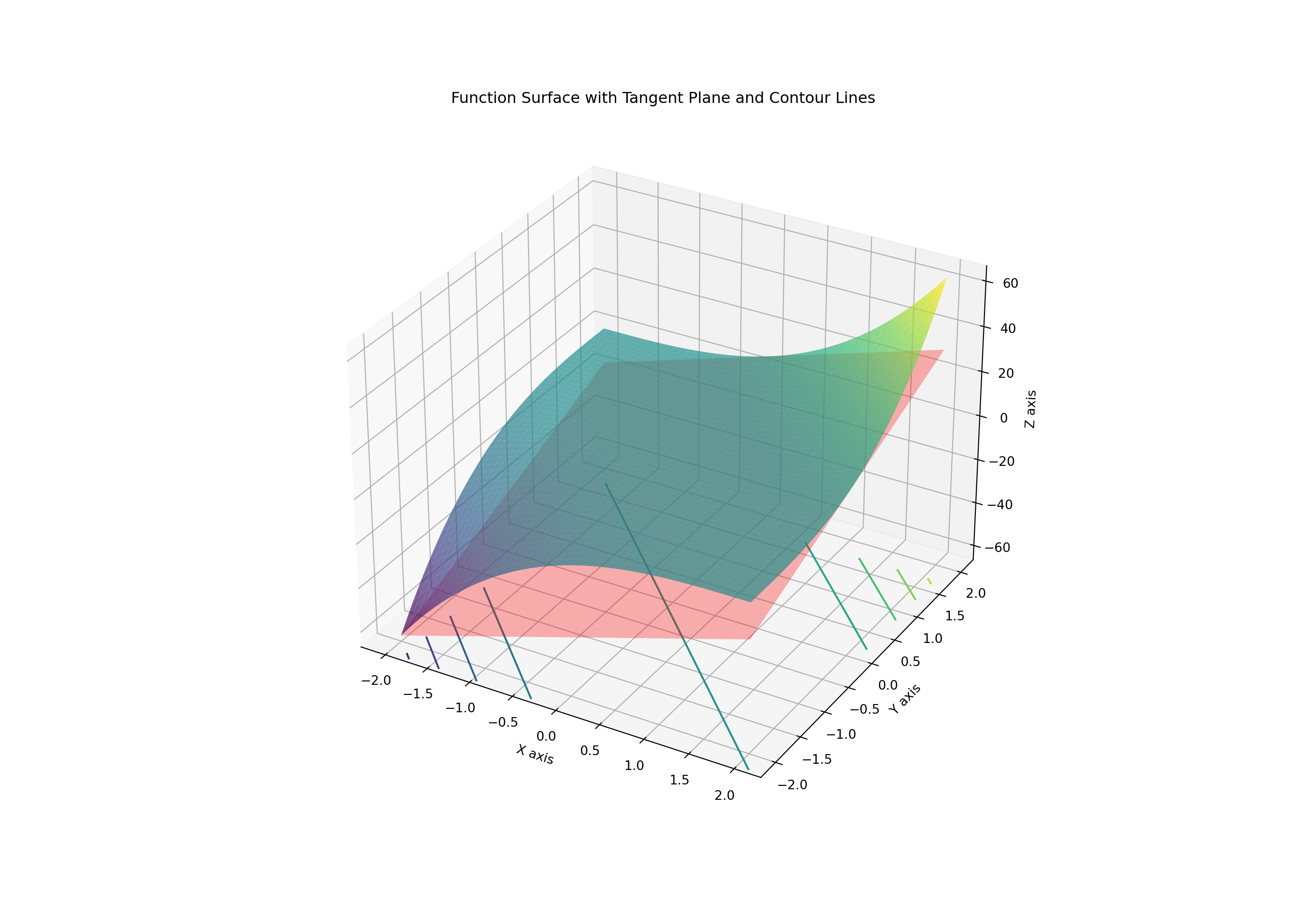

plt.show()

Explanation: To better understand the behavior of the function \(f(x, y)\) and its local approximation, we use the following visualization:

1. Function Surface:
   • The plot shows the surface of the function \(f(x, y) = x^3 + 3x^2y + 3xy^2 + y^3\).
   • This surface illustrates how the function values change over the \(x\) and \(y\) dimensions, providing a three-dimensional view of the function’s behavior.
2. Tangent Plane:
   • The red translucent surface represents the tangent plane at the point \((x_0, y_0) = (1, 1)\).
   • The tangent plane is a local linear approximation of the function’s surface around this point. It is derived from the first-order partial derivatives of the function and provides a way to understand how the function behaves locally.
3. Contour Lines:
   • Contour lines are added to the plot to show lines of constant function value.
   • These lines help visualize the function’s level sets and provide insights into the function’s shape and curvature. They are plotted in the plane of the function surface, giving a sense of how the function’s values change across different regions.

---

3.7.7.1 Problems and Solutions: Second-Order Partial Derivatives

1. Problem 1: Find the second-order partial derivatives of \(f(x, y) = x^3 + 3x^2y + 3xy^2 + y^3\) with respect to \(x\) and \(y\).

   Solution:

   • \(f_x = \frac{\partial}{\partial x}(x^3 + 3x^2y + 3xy^2 + y^3) = 3x^2 + 6xy + 3y^2\)
   • \(f_{xx} = \frac{\partial}{\partial x}(3x^2 + 6xy + 3y^2) = 6x + 6y\)
   • \(f_y = \frac{\partial}{\partial y}(x^3 + 3x^2y + 3xy^2 + y^3) = 3x^2 + 6xy + 3y^2\)
   • \(f_{yy} = \frac{\partial}{\partial y}(3x^2 + 6xy + 3y^2) = 6x + 6y\)
   • \(f_{xy} = \frac{\partial}{\partial y}(3x^2 + 6xy + 3y^2) = 6x + 6y\)
   • \(f_{yx} = \frac{\partial}{\partial x}(3x^2 + 6xy + 3y^2) = 6x + 6y\)

2. Problem 2: Determine the second-order partial derivatives of \(f(x, y) = e^{x^2 + y^2}\).

   Solution:

   • \(f_x = \frac{\partial}{\partial x}(e^{x^2 + y^2}) = 2xe^{x^2 + y^2}\)
   • \(f_{xx} = \frac{\partial}{\partial x}(2xe^{x^2 + y^2}) = 2e^{x^2 + y^2} (2x^2 + 1)\)
   • \(f_y = \frac{\partial}{\partial y}(e^{x^2 + y^2}) = 2ye^{x^2 + y^2}\)
   • \(f_{yy} = \frac{\partial}{\partial y}(2ye^{x^2 + y^2}) = 2e^{x^2 + y^2} (2y^2 + 1)\)
   • \(f_{xy} = \frac{\partial}{\partial y}(2xe^{x^2 + y^2}) = 4xye^{x^2 + y^2}\)
   • \(f_{yx} = \frac{\partial}{\partial x}(2ye^{x^2 + y^2}) = 4xye^{x^2 + y^2}\)

3. Problem 3: Compute the second-order partial derivatives of \(f(x, y) = \sin(xy)\).

   Solution:

   • \(f_x = \frac{\partial}{\partial x}(\sin(xy)) = y \cos(xy)\)
   • \(f_{xx} = \frac{\partial}{\partial x}(y \cos(xy)) = -y^2 \sin(xy)\)
   • \(f_y = \frac{\partial}{\partial y}(\sin(xy)) = x \cos(xy)\)
   • \(f_{yy} = \frac{\partial}{\partial y}(x \cos(xy)) = -x^2 \sin(xy)\)
   • \(f_{xy} = \frac{\partial}{\partial y}(y \cos(xy)) = \cos(xy) - xy \sin(xy)\)
   • \(f_{yx} = \frac{\partial}{\partial x}(x \cos(xy)) = \cos(xy) - xy \sin(xy)\)

4. Problem 4: Find the second-order partial derivatives of \(f(x, y) = \ln(x^2 + y^2)\).

   Solution:

   • \(f_x = \frac{\partial}{\partial x}(\ln(x^2 + y^2)) = \frac{2x}{x^2 + y^2}\)
   • \(f_{xx} = \frac{\partial}{\partial x}\left(\frac{2x}{x^2 + y^2}\right) = \frac{2(y^2 - x^2)}{(x^2 + y^2)^2}\)
   • \(f_y = \frac{\partial}{\partial y}(\ln(x^2 + y^2)) = \frac{2y}{x^2 + y^2}\)
   • \(f_{yy} = \frac{\partial}{\partial y}\left(\frac{2y}{x^2 + y^2}\right) = \frac{2(x^2 - y^2)}{(x^2 + y^2)^2}\)
   • \(f_{xy} = \frac{\partial}{\partial y}\left(\frac{2x}{x^2 + y^2}\right) = -\frac{4xy}{(x^2 + y^2)^2}\)
   • \(f_{yx} = \frac{\partial}{\partial x}\left(\frac{2y}{x^2 + y^2}\right) = -\frac{4xy}{(x^2 + y^2)^2}\)

5. Problem 5: Determine the second-order partial derivatives of \(f(x, y) = \frac{1}{x^2 + y^2 + 1}\).

   Solution:

   • \(f_x = \frac{\partial}{\partial x}\left(\frac{1}{x^2 + y^2 + 1}\right) = -\frac{2x}{(x^2 + y^2 + 1)^2}\)
   • \(f_{xx} = \frac{\partial}{\partial x}\left(-\frac{2x}{(x^2 + y^2 + 1)^2}\right) = \frac{2(3x^2 - y^2 - 1)}{(x^2 + y^2 + 1)^3}\)
   • \(f_y = \frac{\partial}{\partial y}\left(\frac{1}{x^2 + y^2 + 1}\right) = -\frac{2y}{(x^2 + y^2 + 1)^2}\)
   • \(f_{yy} = \frac{\partial}{\partial y}\left(-\frac{2y}{(x^2 + y^2 + 1)^2}\right) = \frac{2(x^2 - 3y^2 - 1)}{(x^2 + y^2 + 1)^3}\)
   • \(f_{xy} = \frac{\partial}{\partial y}\left(-\frac{2x}{(x^2 + y^2 + 1)^2}\right) = \frac{4xy}{(x^2 + y^2 + 1)^3}\)
   • \(f_{yx} = \frac{\partial}{\partial x}\left(-\frac{2y}{(x^2 + y^2 + 1)^2}\right) = \frac{4xy}{(x^2 + y^2 + 1)^3}\)

6. Problem 6: Compute the second-order partial derivatives of \(f(x, y) = \cos(x + y)\).

   Solution:

   • \(f_x = \frac{\partial}{\partial x}(\cos(x + y)) = -\sin(x + y)\)
   • \(f_{xx} = \frac{\partial}{\partial x}(-\sin(x + y)) = -\cos(x + y)\)
   • \(f_y = \frac{\partial}{\partial y}(\cos(x + y)) = -\sin(x + y)\)
   • \(f_{yy} = \frac{\partial}{\partial y}(-\sin(x + y)) = -\cos(x + y)\)
   • \(f_{xy} = \frac{\partial}{\partial y}(-\sin(x + y)) = -\cos(x + y)\)
   • \(f_{yx} = \frac{\partial}{\partial x}(-\sin(x + y)) = -\cos(x + y)\)

7. Problem 7: Find the second-order partial derivatives of \(f(x, y) = x^2 \ln(y)\).

   Solution:

   • \(f_x = \frac{\partial}{\partial x}(x^2 \ln(y)) = 2x \ln(y)\)
   • \(f_{xx} = \frac{\partial}{\partial x}(2x \ln(y)) = 2 \ln(y)\)
   • \(f_y = \frac{\partial}{\partial y}(x^2 \ln(y)) = \frac{x^2}{y}\)
   • \(f_{yy} = \frac{\partial}{\partial y}\left(\frac{x^2}{y}\right) = -\frac{x^2}{y^2}\)
   • \(f_{xy} = \frac{\partial}{\partial y}(2x \ln(y)) = \frac{2x}{y}\)
   • \(f_{yx} = \frac{\partial}{\partial x}\left(\frac{x^2}{y}\right) = \frac{2x}{y}\)

8. Problem 8: Determine the second-order partial derivatives of \(f(x, y) = e^{x} \cdot \cos(y)\).

   Solution:

   • \(f_x = \frac{\partial}{\partial x}(e^x \cdot \cos(y)) = e^x \cdot \cos(y)\)
   • \(f_{xx} = \frac{\partial}{\partial x}(e^x \cdot \cos(y)) = e^x \cdot \cos(y)\)
   • \(f_y = \frac{\partial}{\partial y}(e^x \cdot \cos(y)) = -e^x \cdot \sin(y)\)
   • \(f_{yy} = \frac{\partial}{\partial y}(-e^x \cdot \sin(y)) = -e^x \cdot \cos(y)\)
   • \(f_{xy} = \frac{\partial}{\partial y}(e^x \cdot \cos(y)) = -e^x \cdot \sin(y)\)
   • \(f_{yx} = \frac{\partial}{\partial x}(-e^x \cdot \sin(y)) = -e^x \cdot \sin(y)\)

9. Problem 9: Compute the second-order partial derivatives of \(f(x, y) = x^2 y + e^x\).

   Solution:

   • \(f_x = \frac{\partial}{\partial x}(x^2 y + e^x) = 2xy + e^x\)
   • \(f_{xx} = \frac{\partial}{\partial x}(2xy + e^x) = 2y + e^x\)
   • \(f_y = \frac{\partial}{\partial y}(x^2 y + e^x) = x^2\)
   • \(f_{yy} = \frac{\partial}{\partial y}(x^2) = 0\)
   • \(f_{xy} = \frac{\partial}{\partial y}(2xy + e^x) = 2x\)
   • \(f_{yx} = \frac{\partial}{\partial x}(x^2) = 2x\)

10. Problem 10: Find the second-order partial derivatives of \(f(x, y) = \sqrt{x^2 + y^2}\).

    Solution:

    • \(f_x = \frac{\partial}{\partial x}(\sqrt{x^2 + y^2}) = \frac{x}{\sqrt{x^2 + y^2}}\)
    • \(f_{xx} = \frac{\partial}{\partial x}\left(\frac{x}{\sqrt{x^2 + y^2}}\right) = \frac{y^2}{(x^2 + y^2)^{3/2}}\)
    • \(f_y = \frac{\partial}{\partial y}(\sqrt{x^2 + y^2}) = \frac{y}{\sqrt{x^2 + y^2}}\)
    • \(f_{yy} = \frac{\partial}{\partial y}\left(\frac{y}{\sqrt{x^2 + y^2}}\right) = \frac{x^2}{(x^2 + y^2)^{3/2}}\)
    • \(f_{xy} = \frac{\partial}{\partial y}\left(\frac{x}{\sqrt{x^2 + y^2}}\right) = -\frac{xy}{(x^2 + y^2)^{3/2}}\)
    • \(f_{yx} = \frac{\partial}{\partial x}\left(\frac{y}{\sqrt{x^2 + y^2}}\right) = -\frac{xy}{(x^2 + y^2)^{3/2}}\)

11. Problem 11: Determine the second-order partial derivatives of \(f(x, y) = \arctan(xy)\).

    Solution:

    • \(f_x = \frac{\partial}{\partial x}(\arctan(xy)) = \frac{y}{1 + (xy)^2}\)
    • \(f_{xx} = \frac{\partial}{\partial x}\left(\frac{y}{1 + (xy)^2}\right) = \frac{y^3 x^2 - y}{(1 + x^2 y^2)^2}\)
    • \(f_y = \frac{\partial}{\partial y}(\arctan(xy)) = \frac{x}{1 + (xy)^2}\)
    • \(f_{yy} = \frac{\partial}{\partial y}\left(\frac{x}{1 + (xy)^2}\right) = \frac{x^3 y^2 - x}{(1 + x^2 y^2)^2}\)
    • \(f_{xy} = \frac{\partial}{\partial y}\left(\frac{y}{1 + (xy)^2}\right) = \frac{x (1 - y^2 x^2)}{(1 + x^2 y^2)^2}\)
    • \(f_{yx} = \frac{\partial}{\partial x}\left(\frac{x}{1 + (xy)^2}\right) = \frac{y (1 - x^2 y^2)}{(1 + x^2 y^2)^2}\)

12. Problem 12: Compute the second-order partial derivatives of \(f(x, y) = \frac{x^3 + y^3}{x^2 + y^2 + 1}\).

    Solution:

    • \(f_x = \frac{\partial}{\partial x}\left(\frac{x^3 + y^3}{x^2 + y^2 + 1}\right) = \frac{(3x^2)(x^2 + y^2 + 1) - (x^3 + y^3)(2x)}{(x^2 + y^2 + 1)^2}\)
    • \(f_{xx} = \frac{\partial}{\partial x}\left(\frac{(3x^2)(x^2 + y^2 + 1) - (x^3 + y^3)(2x)}{(x^2 + y^2 + 1)^2}\right) = \frac{6x(x^2 + y^2 + 1) - (3x^2)(2x) - 2(x^3 + y^3) + (2x)(x^3 + y^3)}{(x^2 + y^2 + 1)^3}\)
    • \(f_y = \frac{\partial}{\partial y}\left(\frac{x^3 + y^3}{x^2 + y^2 + 1}\right) = \frac{(3y^2)(x^2 + y^2 + 1) - (x^3 + y^3)(2y)}{(x^2 + y^2 + 1)^2}\)
    • \(f_{yy} = \frac{\partial}{\partial y}\left(\frac{(3y^2)(x^2 + y^2 + 1) - (x^3 + y^3)(2y)}{(x^2 + y^2 + 1)^2}\right) = \frac{6y(x^2 + y^2 + 1) - (3y^2)(2y) - 2(x^3 + y^3) + (2y)(x^3 + y^3)}{(x^2 + y^2 + 1)^3}\)
    • \(f_{xy} = \frac{\partial}{\partial y}\left(\frac{(3x^2)(x^2 + y^2 + 1) - (x^3 + y^3)(2x)}{(x^2 + y^2 + 1)^2}\right) = -\frac{6xy(x^2 + y^2 + 1) - 2(x^3 + y^3) - 2x \cdot (x^3 + y^3)}{(x^2 + y^2 + 1)^3}\)
    • \(f_{yx} = \frac{\partial}{\partial x}\left(\frac{(3y^2)(x^2 + y^2 + 1) - (x^3 + y^3)(2y)}{(x^2 + y^2 + 1)^2}\right) = -\frac{6xy(x^2 + y^2 + 1) - 2(x^3 + y^3) - 2y \cdot (x^3 + y^3)}{(x^2 + y^2 + 1)^3}\)

13. Problem 13: Find the second-order partial derivatives of \(f(x, y) = \tanh(x + y)\).

    Solution:

    • \(f_x = \frac{\partial}{\partial x}(\tanh(x + y)) = \text{sech}^2(x + y)\)
    • \(f_{xx} = \frac{\partial}{\partial x}(\text{sech}^2(x + y)) = -2 \text{sech}^2(x + y) \tanh(x + y)\)
    • \(f_y = \frac{\partial}{\partial y}(\tanh(x + y)) = \text{sech}^2(x + y)\)
    • \(f_{yy} = \frac{\partial}{\partial y}(\text{sech}^2(x + y)) = -2 \text{sech}^2(x + y) \tanh(x + y)\)
    • \(f_{xy} = \frac{\partial}{\partial y}(\text{sech}^2(x + y)) = -2 \text{sech}^2(x + y) \tanh(x + y)\)
    • \(f_{yx} = \frac{\partial}{\partial x}(\text{sech}^2(x + y)) = -2 \text{sech}^2(x + y) \tanh(x + y)\)

14. Problem 14: Determine the second-order partial derivatives of \(f(x, y) = \sin(x^2 + y^2)\).

    Solution:

    • \(f_x = \frac{\partial}{\partial x}(\sin(x^2 + y^2)) = 2x \cos(x^2 + y^2)\)
    • \(f_{xx} = \frac{\partial}{\partial x}(2x \cos(x^2 + y^2)) = 2 \cos(x^2 + y^2) - 4x^2 \sin(x^2 + y^2)\)
    • \(f_y = \frac{\partial}{\partial y}(\sin(x^2 + y^2)) = 2y \cos(x^2 + y^2)\)
    • \(f_{yy} = \frac{\partial}{\partial y}(2y \cos(x^2 + y^2)) = 2 \cos(x^2 + y^2) - 4y^2 \sin(x^2 + y^2)\)
    • \(f_{xy} = \frac{\partial}{\partial y}(2x \cos(x^2 + y^2)) = -4xy \sin(x^2 + y^2)\)
    • \(f_{yx} = \frac{\partial}{\partial x}(2y \cos(x^2 + y^2)) = -4xy \sin(x^2 + y^2)\)

15. Problem 15: Compute the second-order partial derivatives of \(f(x, y) = \frac{\sin(x + y)}{x^2 + y^2 + 1}\).

    Solution:

    • \(f_x = \frac{\partial}{\partial x}\left(\frac{\sin(x + y)}{x^2 + y^2 + 1}\right) = \frac{\cos(x + y) (x^2 + y^2 + 1) - \sin(x + y) \cdot 2x}{(x^2 + y^2 + 1)^2}\)
    • \(f_{xx} = \frac{\partial}{\partial x}\left(\frac{\cos(x + y) (x^2 + y^2 + 1) - \sin(x + y) \cdot 2x}{(x^2 + y^2 + 1)^2}\right) = \frac{-\sin(x + y)(x^2 + y^2 + 1) - 2\cos(x + y)(x^2 + y^2 + 1) - 2\cos(x + y) \cdot 2x + 2\sin(x + y) \cdot 2x}{(x^2 + y^2 + 1)^3}\)
    • \(f_y = \frac{\partial}{\partial y}\left(\frac{\sin(x + y)}{x^2 + y^2 + 1}\right) = \frac{\cos(x + y) (x^2 + y^2 + 1) - \sin(x + y) \cdot 2y}{(x^2 + y^2 + 1)^2}\)
    • \(f_{yy} = \frac{\partial}{\partial y}\left(\frac{\cos(x + y) (x^2 + y^2 + 1) - \sin(x + y) \cdot 2y}{(x^2 + y^2 + 1)^2}\right) = \frac{-\sin(x + y)(x^2 + y^2 + 1) - 2\cos(x + y)(x^2 + y^2 + 1) - 2\cos(x + y) \cdot 2y + 2\sin(x + y) \cdot 2y}{(x^2 + y^2 + 1)^3}\)
    • \(f_{xy} = \frac{\partial}{\partial y}\left(\frac{\cos(x + y) (x^2 + y^2 + 1) - \sin(x + y) \cdot 2x}{(x^2 + y^2 + 1)^2}\right) = \frac{-\sin(x + y)(x^2 + y^2 + 1) - \cos(x + y) \cdot 2x - 2\cos(x + y) \cdot 2y + 2\sin(x + y) \cdot 2x}{(x^2 + y^2 + 1)^3}\)
    • \(f_{yx} = \frac{\partial}{\partial x}\left(\frac{\cos(x + y) (x^2 + y^2 + 1) - \sin(x + y) \cdot 2y}{(x^2 + y^2 + 1)^2}\right) = \frac{-\sin(x + y)(x^2 + y^2 + 1) - \cos(x + y) \cdot 2y - 2\cos(x + y) \cdot 2x + 2\sin(x + y) \cdot 2y}{(x^2 + y^2 + 1)^3}\)

16. Problem 16: Find the second-order partial derivatives of \(f(x, y) = x^2 \cdot y^2\).

    Solution:

    • \(f_x = \frac{\partial}{\partial x}(x^2 y^2) = 2x y^2\)
    • \(f_{xx} = \frac{\partial}{\partial x}(2x y^2) = 2 y^2\)
    • \(f_y = \frac{\partial}{\partial y}(x^2 y^2) = 2x^2 y\)
    • \(f_{yy} = \frac{\partial}{\partial y}(2x^2 y) = 2x^2\)
    • \(f_{xy} = \frac{\partial}{\partial y}(2x y^2) = 4x y\)
    • \(f_{yx} = \frac{\partial}{\partial x}(2x y^2) = 4x y\)

17. Problem 17: Determine the second-order partial derivatives of \(f(x, y) = \ln(x^2 + y^2 + 1)\).

    Solution:

    • \(f_x = \frac{\partial}{\partial x}(\ln(x^2 + y^2 + 1)) = \frac{2x}{x^2 + y^2 + 1}\)
    • \(f_{xx} = \frac{\partial}{\partial x}\left(\frac{2x}{x^2 + y^2 + 1}\right) = \frac{2(y^2 - x^2 + 1)}{(x^2 + y^2 + 1)^2}\)
    • \(f_y = \frac{\partial}{\partial y}(\ln(x^2 + y^2 + 1)) = \frac{2y}{x^2 + y^2 + 1}\)
    • \(f_{yy} = \frac{\partial}{\partial y}\left(\frac{2y}{x^2 + y^2 + 1}\right) = \frac{2(x^2 - y^2 + 1)}{(x^2 + y^2 + 1)^2}\)
    • \(f_{xy} = \frac{\partial}{\partial y}\left(\frac{2x}{x^2 + y^2 + 1}\right) = -\frac{4xy}{(x^2 + y^2 + 1)^2}\)
    • \(f_{yx} = \frac{\partial}{\partial x}\left(\frac{2y}{x^2 + y^2 + 1}\right) = -\frac{4xy}{(x^2 + y^2 + 1)^2}\)

18. Problem 18: Compute the second-order partial derivatives of \(f(x, y) = \sqrt{1 + x^2 - y^2}\).

    Solution:

    • \(f_x = \frac{\partial}{\partial x}\left(\sqrt{1 + x^2 - y^2}\right) = \frac{x}{\sqrt{1 + x^2 - y^2}}\)
    • \(f_{xx} = \frac{\partial}{\partial x}\left(\frac{x}{\sqrt{1 + x^2 - y^2}}\right) = \frac{1 - x^2 + y^2}{(1 + x^2 - y^2)^{3/2}}\)
    • \(f_y = \frac{\partial}{\partial y}\left(\sqrt{1 + x^2 - y^2}\right) = \frac{-y}{\sqrt{1 + x^2 - y^2}}\)
    • \(f_{yy} = \frac{\partial}{\partial y}\left(\frac{-y}{\sqrt{1 + x^2 - y^2}}\right) = \frac{x^2 - 1 + y^2}{(1 + x^2 - y^2)^{3/2}}\)
    • \(f_{xy} = \frac{\partial}{\partial y}\left(\frac{x}{\sqrt{1 + x^2 - y^2}}\right) = \frac{xy}{(1 + x^2 - y^2)^{3/2}}\)
    • \(f_{yx} = \frac{\partial}{\partial x}\left(\frac{-y}{\sqrt{1 + x^2 - y^2}}\right) = \frac{xy}{(1 + x^2 - y^2)^{3/2}}\)

Problem 19: Compute the second-order partial derivatives of \(f(x, y) = \sqrt{x^2 + y^2}\).

Solution:

• First-order partial derivatives: \[ f_x = \frac{x}{\sqrt{x^2 + y^2}} \] \[ f_y = \frac{y}{\sqrt{x^2 + y^2}} \]

• Second-order partial derivatives: \[ f_{xx} = \frac{y^2}{(x^2 + y^2)^{3/2}} \] \[ f_{yy} = \frac{x^2}{(x^2 + y^2)^{3/2}} \] \[ f_{xy} = -\frac{xy}{(x^2 + y^2)^{3/2}} \] \[ f_{yx} = -\frac{xy}{(x^2 + y^2)^{3/2}} \]

Problem 20: Find the second-order partial derivatives of \(f(x, y) = x^3 - 3x^2y + 2xy^2\).

Solution:

• First-order partial derivatives: \[ f_x = 3x^2 - 6xy + 2y^2 \] \[ f_y = -3x^2 + 4xy \]

• Second-order partial derivatives: \[ f_{xx} = 6x - 6y \] \[ f_{yy} = 4x \] \[ f_{xy} = -6x + 4y \] \[ f_{yx} = -6x + 4y \] Problem 21: In a manufacturing process, the temperature \(T\) at a point \((x, y)\) in a metal plate is given by \(T(x, y) = 100 - x^2 - y^2\). Determine the rate of change of temperature at the point \((1, 1)\) in the direction of the x-axis and y-axis.

Solution:

• First-order partial derivatives: \[ T_x = -2x \] \[ T_y = -2y \]

• At point \((1, 1)\): \[ T_x(1, 1) = -2 \] \[ T_y(1, 1) = -2 \]

  The rate of change of temperature in the x-direction is \(-2\) and in the y-direction is \(-2\).

3.7.8 Summary of Concepts

In this module, we explored several key concepts related to functions of multiple variables, their properties, and applications. We began with an introduction to functions of several variables, where we defined functions that depend on more than one variable, such as \(f(x, y)\). We then discussed the graph of a function, level sets, and projections, providing visual representations in 3D space. The relationship between level sets and contours was also covered, with contours representing lines on a 2D plot where the function has the same value.

We delved into the limits and continuity for functions of two variables, extending the concepts from single-variable calculus. Limits for bivariate functions were discussed, considering multiple paths and providing visual examples. We defined continuity formally, ensuring the function is defined at a point, the limit exists, and the limit equals the function’s value at that point. The concepts of partial derivatives and higher-order derivatives were introduced, with first-order partial derivatives representing the rate of change in one direction and second-order partial derivatives representing the curvature of the function.

Convexity and concavity were discussed, with mathematical tools like second-order partial derivatives used to determine the curvature of functions. Finally, we provided various practical problems and solutions involving higher-order derivatives, partial derivatives, limits, continuity, and linearization to illustrate their applications in engineering and computer science contexts.

3.8 Module-3 Calculus for analysis and un-constrined optimization

Syllabus Content: The Chain Rule, Directional Derivatives in the Plane, Interpretation of the Directional Derivative, Gradient, Properties of the Directional Derivative, Relative extrema, Second Derivative Test for Local Extreme Values, Absolute Maxima and Minima.(Total 9 hours)

---

3.8.1 Introduction

In this module, we delve into the practical applications of calculus in the fields of computer science and engineering. Calculus, particularly multivariable calculus, plays a crucial role in understanding and solving complex problems that arise in these disciplines. We will explore several advanced topics and their applications, providing a comprehensive understanding of how these mathematical concepts can be utilized effectively.

We begin with the Chain Rule, which is essential for differentiating composite functions and is widely used in various algorithms and computations. Next, we introduce Directional Derivatives in the Plane, which measure the rate of change of a function in any given direction. This leads to an understanding of the Interpretation of the Directional Derivative, providing insights into how functions behave in different directions.

The Gradient of a function is then discussed, representing the vector of partial derivatives and indicating the direction of the steepest ascent. We explore the Properties of the Directional Derivative to understand how it relates to the gradient and its significance in optimization problems.

Moving forward, we examine Relative Extrema, identifying points where a function takes on local maximum or minimum values. The Second Derivative Test for Local Extreme Values is introduced as a method to classify these extrema. Finally, we discuss Absolute Maxima and Minima, determining the highest and lowest values a function can attain within a given domain.

Throughout this module, we will provide practical examples and problems to illustrate these concepts, ensuring a solid grasp of their applications in real-world scenarios in computer science and engineering. By the end of this module, you will be equipped with the necessary tools to apply advanced calculus techniques to solve complex problems in your field.

3.8.2 Chain rule in differentiation

In the study of multivariable calculus, the Chain Rule is a fundamental tool for differentiating composite functions. This rule is particularly important in computer science and engineering, where functions are often composed of multiple variables and their relationships are intricate.

Definition: The Chain Rule provides a method to differentiate a composite function. If we have two functions \(u = g(t)\) and \(y = f(u)\), then the composite function \(y = f(g(t))\) can be differentiated using the Chain Rule. Mathematically, it is expressed as:

\[ \frac{dy}{dt} = \frac{dy}{du} \cdot \frac{du}{dt} \]

For functions of several variables, the Chain Rule generalizes to handle compositions of functions of multiple variables. Suppose \(z = f(x, y)\), where \(x = g(t)\) and \(y = h(t)\). Then, the derivative of \(z\) with respect to \(t\) is given by:

\[ \frac{dz}{dt} = \frac{\partial f}{\partial x} \cdot \frac{dx}{dt} + \frac{\partial f}{\partial y} \cdot \frac{dy}{dt} \]

Example:

Consider a temperature distribution function \(T(x, y)\), where \(T\) represents temperature at a point \((x, y)\) in a plane. Suppose the coordinates \((x, y)\) depend on time \(t\), such that \(x = t^2\) and \(y = \sin(t)\). To find how the temperature changes over time, we apply the Chain Rule.

First, calculate the partial derivatives:

\[ \frac{\partial T}{\partial x} \quad \text{and} \quad \frac{\partial T}{\partial y} \]

Next, compute the derivatives of \(x\) and \(y\) with respect to \(t\):

\[ \frac{dx}{dt} = 2t \quad \text{and} \quad \frac{dy}{dt} = \cos(t) \]

Finally, apply the Chain Rule:

\[ \frac{dT}{dt} = \frac{\partial T}{\partial x} \cdot \frac{dx}{dt} + \frac{\partial T}{\partial y} \cdot \frac{dy}{dt} = \frac{\partial T}{\partial x} \cdot 2t + \frac{\partial T}{\partial y} \cdot \cos(t) \]

In this example, the Chain Rule allows us to understand how temperature changes over time based on the movement of coordinates.

Similarly, if \(z = f(x, y)\) where \(x = g(\theta, \phi)\) and \(y = h(\theta, \phi)\), then the partial derivatives of \(z\) with respect to \(\theta\) and \(\phi\) are given by:

\[ \frac{\partial z}{\partial \theta} = \frac{\partial f}{\partial x} \cdot \frac{\partial x}{\partial \theta} + \frac{\partial f}{\partial y} \cdot \frac{\partial y}{\partial \theta} \]

\[ \frac{\partial z}{\partial \phi} = \frac{\partial f}{\partial x} \cdot \frac{\partial x}{\partial \phi} + \frac{\partial f}{\partial y} \cdot \frac{\partial y}{\partial \phi} \]

Example for the Second Case of Chain Rule:

Consider a scenario where we have a function \(z = f(x, y)\) that depends on two intermediate variables \(x\) and \(y\), which in turn depend on two other variables \(\theta\) and \(\phi\). This is common in applications where transformations or parameterizations are involved.

Let’s take the following functions: \[ z = f(x, y) = x^2 + y^2 \] \[ x = g(\theta, \phi) = \theta + \phi \] \[ y = h(\theta, \phi) = \theta \phi \]

We want to find the partial derivatives of \(z\) with respect to \(\theta\) and \(\phi\).

Step-by-Step Solution:

1. Calculate the partial derivatives of \(f(x, y)\):

   \[ \frac{\partial f}{\partial x} = 2x \quad \text{and} \quad \frac{\partial f}{\partial y} = 2y \]

2. Compute the partial derivatives of \(x\) and \(y\) with respect to \(\theta\):

   \[ \frac{\partial x}{\partial \theta} = 1 \quad \text{and} \quad \frac{\partial y}{\partial \theta} = \phi \]

3. Compute the partial derivatives of \(x\) and \(y\) with respect to \(\phi\):

   \[ \frac{\partial x}{\partial \phi} = 1 \quad \text{and} \quad \frac{\partial y}{\partial \phi} = \theta \]

4. Apply the Chain Rule to find the partial derivatives of \(z\):

   For \(\theta\):

   \[ \frac{\partial z}{\partial \theta} = \frac{\partial f}{\partial x} \cdot \frac{\partial x}{\partial \theta} + \frac{\partial f}{\partial y} \cdot \frac{\partial y}{\partial \theta} \] \[ \frac{\partial z}{\partial \theta} = 2x \cdot 1 + 2y \cdot \phi \]

   Substituting \(x = \theta + \phi\) and \(y = \theta \phi\):

   \[ \frac{\partial z}{\partial \theta} = 2(\theta + \phi) + 2(\theta \phi) \cdot \phi \] \[ \frac{\partial z}{\partial \theta} = 2\theta + 2\phi + 2\theta \phi^2 \]

   For \(\phi\):

   \[ \frac{\partial z}{\partial \phi} = \frac{\partial f}{\partial x} \cdot \frac{\partial x}{\partial \phi} + \frac{\partial f}{\partial y} \cdot \frac{\partial y}{\partial \phi} \] \[ \frac{\partial z}{\partial \phi} = 2x \cdot 1 + 2y \cdot \theta \]

   Substituting \(x = \theta + \phi\) and \(y = \theta \phi\):

   \[ \frac{\partial z}{\partial \phi} = 2(\theta + \phi) + 2(\theta \phi) \cdot \theta \] \[ \frac{\partial z}{\partial \phi} = 2\theta + 2\phi + 2\theta^2 \phi \]

Summary:

The partial derivatives of \(z = f(x, y) = x^2 + y^2\) with respect to \(\theta\) and \(\phi\), given the intermediate dependencies \(x = g(\theta, \phi) = \theta + \phi\) and \(y = h(\theta, \phi) = \theta \phi\), are:

\[ \frac{\partial z}{\partial \theta} = 2\theta + 2\phi + 2\theta \phi^2 \] \[ \frac{\partial z}{\partial \phi} = 2\theta + 2\phi + 2\theta^2 \phi \]

Physical Meaning:

In this context, the function \(z\) could represent a physical quantity such as energy, cost, or some other measure that depends on intermediate variables \(x\) and \(y\). The variables \(\theta\) and \(\phi\) might represent parameters like time or spatial coordinates. The partial derivatives \(\frac{\partial z}{\partial \theta}\) and \(\frac{\partial z}{\partial \phi}\) describe how the quantity \(z\) changes with respect to these parameters. For instance, if \(\theta\) represents time, \(\frac{\partial z}{\partial \theta}\) would tell us how \(z\) changes over time, considering the indirect effects through \(x\) and \(y\). This type of analysis is crucial in engineering and computational applications for understanding and optimizing system behaviors.

Example 3:

Consider a function \(z = f(x, y) = x^2 + y^2\), where the variables \(x\) and \(y\) are themselves functions of other variables \(\theta\) and \(\phi\): \[ x = g(\theta, \phi) = \theta + \phi \] \[ y = h(\theta, \phi) = \theta \phi \]

To find the partial derivatives of \(z\) with respect to \(\theta\) and \(\phi\), we use the chain rule.

Applying the Chain Rule:

The chain rule states: \[ \frac{\partial z}{\partial \theta} = \frac{\partial z}{\partial x} \cdot \frac{\partial x}{\partial \theta} + \frac{\partial z}{\partial y} \cdot \frac{\partial y}{\partial \theta} \] \[ \frac{\partial z}{\partial \phi} = \frac{\partial z}{\partial x} \cdot \frac{\partial x}{\partial \phi} + \frac{\partial z}{\partial y} \cdot \frac{\partial y}{\partial \phi} \]

First, compute the intermediate partial derivatives: \[ \frac{\partial z}{\partial x} = 2x \] \[ \frac{\partial z}{\partial y} = 2y \] \[ \frac{\partial x}{\partial \theta} = 1 \] \[ \frac{\partial x}{\partial \phi} = 1 \] \[ \frac{\partial y}{\partial \theta} = \phi \] \[ \frac{\partial y}{\partial \phi} = \theta \]

Now, plug these into the chain rule equations: \[ \frac{\partial z}{\partial \theta} = 2x \cdot 1 + 2y \cdot \phi = 2(\theta + \phi) + 2(\theta \phi) \cdot \phi = 2(\theta + \phi) + 2\theta \phi^2 \] \[ \frac{\partial z}{\partial \phi} = 2x \cdot 1 + 2y \cdot \theta = 2(\theta + \phi) + 2(\theta \phi) \cdot \theta = 2(\theta + \phi) + 2\theta^2 \phi \]

Visualization of the Function and its Partial Derivatives

Here is the Python code to visualize the function \(z\), its partial derivatives with respect to \(\theta\) and \(\phi\), and the corresponding contour plot:

import numpy as np
import matplotlib.pyplot as plt
from mpl_toolkits.mplot3d import Axes3D

# Define the functions
def f(x, y):
    return x**2 + y**2

def g(theta, phi):
    return theta + phi

def h(theta, phi):
    return theta * phi

# Generate theta and phi values
theta = np.linspace(-2, 2, 400)
phi = np.linspace(-2, 2, 400)
theta, phi = np.meshgrid(theta, phi)

# Compute x and y
x = g(theta, phi)
y = h(theta, phi)

# Compute z
z = f(x, y)

# Compute partial derivatives
df_dtheta = 2*(theta + phi) + 2*theta * phi**2
df_dphi = 2*(theta + phi) + 2*theta**2 * phi

# Create the 3D plot
fig = plt.figure(figsize=(12, 8))
ax = fig.add_subplot(111, projection='3d')

# Plot the surface
surface = ax.plot_surface(theta, phi, z, cmap='viridis', edgecolor='red', alpha=0.6)

# Plot the contours
contour = ax.contour(theta, phi, z, zdir='z', offset=-1, cmap='viridis')

# Plot the partial derivatives
#ax.quiver(theta, phi, z, df_dtheta, df_dphi, np.zeros_like(z), length=0.1, color='green')

# Labels
ax.set_xlabel('Theta')

## Text(0.5, 0, 'Theta')

ax.set_ylabel('Phi')

## Text(0.5, 0.5, 'Phi')

ax.set_zlabel('z')

## Text(0.5, 0, 'z')

# Title
ax.set_title('Visualization of z=f(x,y)=x^2+y^2 with partial derivatives')

## Text(0.5, 0.92, 'Visualization of z=f(x,y)=x^2+y^2 with partial derivatives')

# Show color bar
fig.colorbar(surface, shrink=0.5, aspect=5)

## <matplotlib.colorbar.Colorbar object at 0x0000029F569E9490>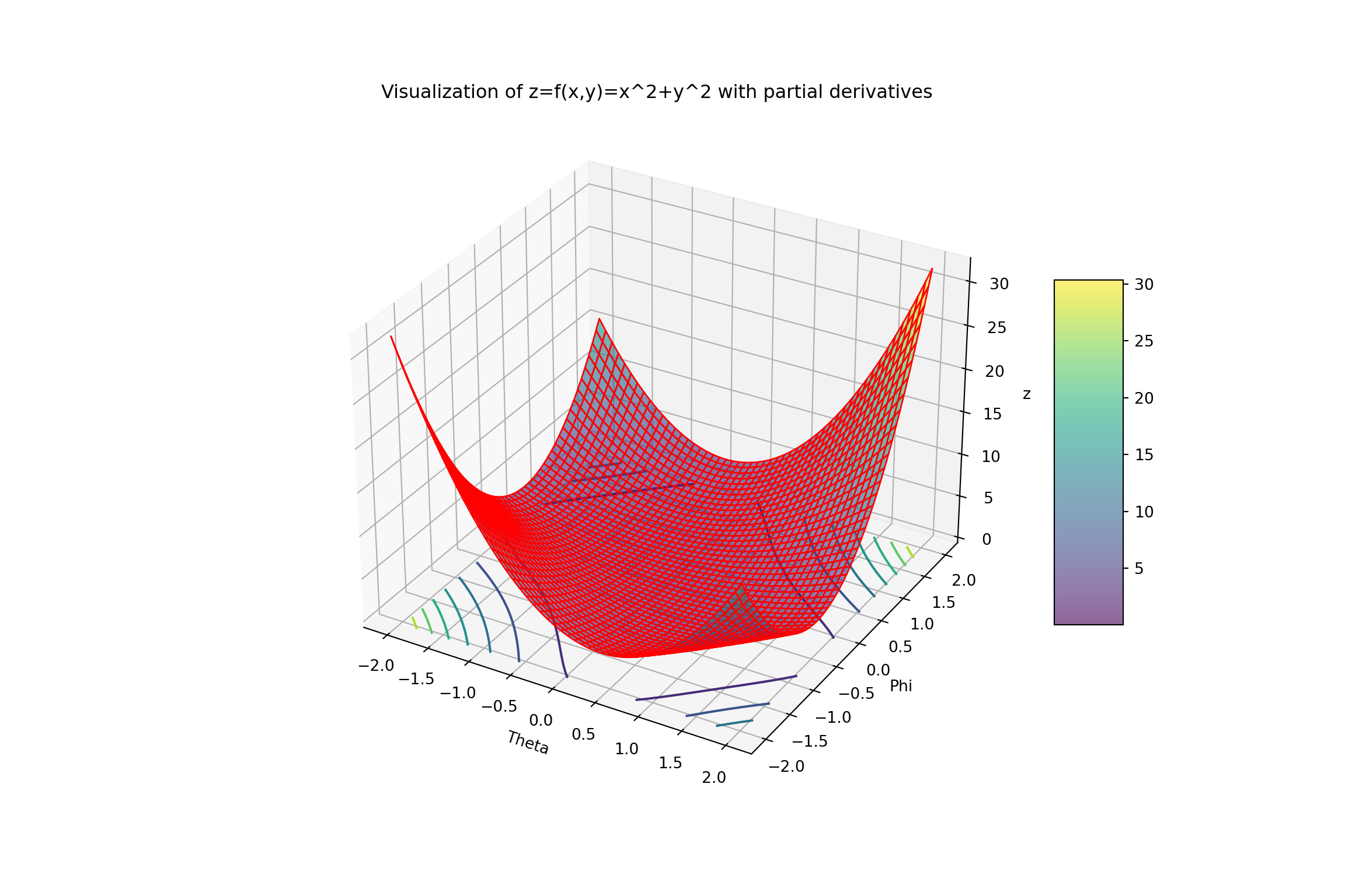

# Show the plot
plt.show()

Interpretation of the mdoel: The surface plot represents the function \(z = x^2 + y^2\) where \(x = \theta + \phi\) and \(y = \theta \phi\). The red arrows indicate the partial derivatives with respect to \(\theta\) and \(\phi\), showing the direction and rate of change of the function as the parameters vary. The contour lines on the plane provide a top-down view of how \(z\) changes with \(\theta\) and \(\phi\).

Physical Meaning: In a physical context, the partial derivatives represent how the output of the function \(z\) changes as you make small changes in the input parameters \(\theta\) and \(\phi\). This can be visualized as the slope of the surface in the direction of each parameter. For example, in a computer graphics scenario, this could represent how changes in position (parameterized by \(\theta\) and \(\phi\)) affect the intensity or color value \(z\) at a particular pixel.

The Chain Rule is extensively used in various applications, such as in neural networks for backpropagation, where it helps in calculating gradients efficiently. It also plays a crucial role in optimization algorithms, control systems, and other computational methods in engineering.

3.8.3 Gradient of a Scalar Field and Its Importance

The gradient of a scalar field is useful in various applications in engineering and computer science. It extends the idea of a derivative to functions of several variables, providing a vector that points in the direction of the greatest rate of increase of the function.

Definition: For a scalar function \(f(x, y)\), the gradient is a vector-valued function denoted by \(\nabla f\) and is defined as:

\[ \nabla f(x, y) = \left\langle \frac{\partial f}{\partial x}, \frac{\partial f}{\partial y} \right\rangle \]

In three dimensions, for a function \(f(x, y, z)\), the gradient is:

\[ \nabla f(x, y, z) = \left\langle \frac{\partial f}{\partial x}, \frac{\partial f}{\partial y}, \frac{\partial f}{\partial z} \right\rangle \]

The components of the gradient vector are the partial derivatives of \(f\) with respect to each variable.

3.8.3.1 Practice Problems

1. Problem 1: Find the gradient of \(f(x, y) = 3x^2y - 2xy^2\) at the point \((1, -1)\).

   Solution: \[ \frac{\partial f}{\partial x} = 6xy - 2y^2 \] \[ \frac{\partial f}{\partial y} = 3x^2 - 4xy \] At \((1, -1)\): \[ \frac{\partial f}{\partial x} = 6(1)(-1) - 2(-1)^2 = -6 - 2 = -8 \] \[ \frac{\partial f}{\partial y} = 3(1)^2 - 4(1)(-1) = 3 + 4 = 7 \] Gradient at \((1, -1)\) is \((-8, 7)\).

2. Problem 2: Find the gradient of \(f(x, y) = e^x \sin(y)\) at the point \((0, \frac{\pi}{2})\).

   Solution: \[ \frac{\partial f}{\partial x} = e^x \sin(y) \] \[ \frac{\partial f}{\partial y} = e^x \cos(y) \] At \((0, \frac{\pi}{2})\): \[ \frac{\partial f}{\partial x} = e^0 \sin(\frac{\pi}{2}) = 1 \] \[ \frac{\partial f}{\partial y} = e^0 \cos(\frac{\pi}{2}) = 0 \] Gradient at \((0, \frac{\pi}{2})\) is \((1, 0)\).

3. Problem 3: Find the gradient of \(f(x, y) = \ln(x^2 + y^2 + 1)\) at the point \((1, 1)\).

   Solution: \[ \frac{\partial f}{\partial x} = \frac{2x}{x^2 + y^2 + 1} \] \[ \frac{\partial f}{\partial y} = \frac{2y}{x^2 + y^2 + 1} \] At \((1, 1)\): \[ \frac{\partial f}{\partial x} = \frac{2(1)}{1^2 + 1^2 + 1} = \frac{2}{3} \] \[ \frac{\partial f}{\partial y} = \frac{2(1)}{1^2 + 1^2 + 1} = \frac{2}{3} \] Gradient at \((1, 1)\) is \(\left(\frac{2}{3}, \frac{2}{3}\right)\).

4. Problem 4: Find the gradient of \(f(x, y) = x^3 - 3xy + y^3\) at the point \((2, -1)\).

   Solution: \[ \frac{\partial f}{\partial x} = 3x^2 - 3y \] \[ \frac{\partial f}{\partial y} = -3x + 3y^2 \] At \((2, -1)\): \[ \frac{\partial f}{\partial x} = 3(2)^2 - 3(-1) = 12 + 3 = 15 \] \[ \frac{\partial f}{\partial y} = -3(2) + 3(-1)^2 = -6 + 3 = -3 \] Gradient at \((2, -1)\) is \((15, -3)\).

5. Problem 5: Find the gradient of \(f(x, y) = \sqrt{x^2 + y^2}\) at the point \((3, 4)\).

   Solution: \[ \frac{\partial f}{\partial x} = \frac{x}{\sqrt{x^2 + y^2}} \] \[ \frac{\partial f}{\partial y} = \frac{y}{\sqrt{x^2 + y^2}} \] At \((3, 4)\): \[ \frac{\partial f}{\partial x} = \frac{3}{\sqrt{3^2 + 4^2}} = \frac{3}{5} \] \[ \frac{\partial f}{\partial y} = \frac{4}{\sqrt{3^2 + 4^2}} = \frac{4}{5} \] Gradient at \((3, 4)\) is \(\left(\frac{3}{5}, \frac{4}{5}\right)\).

6. Problem 6: Find the gradient of \(f(x, y) = \frac{x^2 + y^2}{x - y}\) at the point \((1, 2)\).

   Solution: \[ \frac{\partial f}{\partial x} = \frac{(2x(x - y) - (x^2 + y^2))}{(x - y)^2} \] \[ \frac{\partial f}{\partial y} = \frac{(2y(x - y) + (x^2 + y^2))}{(x - y)^2} \] At \((1, 2)\): \[ \frac{\partial f}{\partial x} = \frac{1^2 + 2^2 - 2(1)(2)}{(1 - 2)^2} = \frac{1 + 4 - 4}{1} = 1 \] \[ \frac{\partial f}{\partial y} = \frac{2(1)(2) - 1^2 - 2^2}{(1 - 2)^2} = \frac{4 - 1 - 4}{1} = -1 \] Gradient at \((1, 2)\) is \((1, -1)\).

7. Problem 7: Find the gradient of \(f(x, y) = \cos(x) \cdot \sin(y)\) at the point \((\frac{\pi}{2}, \frac{\pi}{2})\).

   Solution: \[ \frac{\partial f}{\partial x} = -\sin(x) \sin(y) \] \[ \frac{\partial f}{\partial y} = \cos(x) \cos(y) \] At \((\frac{\pi}{2}, \frac{\pi}{2})\): \[ \frac{\partial f}{\partial x} = -\sin(\frac{\pi}{2}) \sin(\frac{\pi}{2}) = -1 \] \[ \frac{\partial f}{\partial y} = \cos(\frac{\pi}{2}) \cos(\frac{\pi}{2}) = 0 \] Gradient at \((\frac{\pi}{2}, \frac{\pi}{2})\) is \((-1, 0)\).

8. Problem 8: Find the gradient of \(f(x, y) = x \exp(y)\) at the point \((1, 0)\).

   Solution: \[ \frac{\partial f}{\partial x} = \exp(y) \] \[ \frac{\partial f}{\partial y} = x \exp(y) \] At \((1, 0)\): \[ \frac{\partial f}{\partial x} = \exp(0) = 1 \] \[ \frac{\partial f}{\partial y} = 1 \cdot \exp(0) = 1 \] Gradient at \((1, 0)\) is \((1, 1)\).

9. Problem 9: Find the gradient of \(f(x, y) = \frac{1}{x^2 + y^2 + 1}\) at the point \((0, 0)\).

   Solution: \[ \frac{\partial f}{\partial x} = \frac{-2x}{(x^2 + y^2 + 1)^2} \] \[ \frac{\partial f}{\partial y} = \frac{-2y}{(x^2 + y^2 + 1)^2} \] At \((0, 0)\): \[ \frac{\partial f}{\partial x} = \frac{-2(0)}{(0^2 + 0^2 + 1)^2} = 0 \] \[ \frac{\partial f}{\partial y} = \frac{-2(0)}{(0^2 + 0^2 + 1)^2} = 0 \] Gradient at \((0, 0)\) is \((0, 0)\).

10. Problem 10: Find the gradient of \(f(x, y) = x^2 e^y\) at the point \((2, 1)\).

Solution: \[ \frac{\partial f}{\partial x} = 2x e^y \] \[ \frac{\partial f}{\partial y} = x^2 e^y \] At \((2, 1)\): \[ \frac{\partial f}{\partial x} = 2(2) e^1 = 4e \] \[ \frac{\partial f}{\partial y} = (2)^2 e^1 = 4e \] Gradient at \((2, 1)\) is \((4e, 4e)\).

3.8.3.2 Importance of the Gradient

1. Direction of Maximum Increase: The gradient vector points in the direction where the function increases most rapidly. This is crucial in optimization problems, where finding the maximum or minimum values of a function is necessary.

2. Magnitude of Change: The magnitude of the gradient vector indicates the rate of increase in that direction. A larger magnitude means a steeper slope.

3. Normal to Level Sets: The gradient vector is perpendicular (normal) to the level sets (contour lines) of the function. This property is used in computer graphics for shading and rendering surfaces.

4. Applications in Machine Learning: In machine learning, the gradient is used in algorithms like gradient descent to minimize cost functions, thus optimizing models.

3.8.3.3 Properties of the Gradient

1. Linearity: The gradient operator is linear. For scalar functions \(f\) and \(g\) and scalars \(a\) and \(b\):

\[ \nabla (a f + b g) = a \nabla f + b \nabla g \]

2. Product Rule: For scalar functions \(f\) and \(g\):

\[ \nabla (f g) = f \nabla g + g \nabla f \]

3. Chain Rule: If \(f\) is a function of \(u\), which is a function of \(x\) and \(y\):

\[ \nabla f(u(x, y)) = \frac{d f}{d u} \nabla u(x, y) \]

4. Gradient and Divergence: The divergence of the gradient of \(f\), known as the Laplacian, is:

\[ \nabla \cdot (\nabla f) = \Delta f \]

Example: Gradient of \(z = x^2 + y^2\)

Consider the function \(z = x^2 + y^2\). Let’s compute and interpret the gradient.

\[ \nabla f(x, y) = \left\langle \frac{\partial z}{\partial x}, \frac{\partial z}{\partial y} \right\rangle = \left\langle 2x, 2y \right\rangle \]

At the point \((1, 1)\):

\[ \nabla f(1, 1) = \left\langle 2 \cdot 1, 2 \cdot 1 \right\rangle = \langle 2, 2 \rangle \]

This gradient vector \(\langle 2, 2 \rangle\) points in the direction of the steepest increase of the function \(z = x^2 + y^2\) at the point \((1, 1)\), and its magnitude indicates the rate of increase.

Visualization

The plot below illustrates the function \(z = x^2 + y^2\), its gradient vectors at various points, and the specific gradient vector at \((1, 1)\).

import numpy as np
import matplotlib.pyplot as plt
from mpl_toolkits.mplot3d import Axes3D

# Define the function
def f(x, y):
    return x**2 + y**2

# Define the gradient
def grad_f(x, y):
    return np.array([2*x, 2*y])

# Define the points and the direction vector
x0, y0 = 1, 1
u = np.array([3, 4])
u = u / np.linalg.norm(u)  # Normalize the direction vector

# Create the grid for plotting
x = np.linspace(-3, 3, 100)
y = np.linspace(-3, 3, 100)
x, y = np.meshgrid(x, y)
z = f(x, y)

# Plot the surface
fig = plt.figure()
ax = fig.add_subplot(111, projection='3d')
ax.plot_surface(x, y, z, cmap='viridis', edgecolor='red', alpha=0.4)

## <mpl_toolkits.mplot3d.art3d.Poly3DCollection object at 0x0000029F5934D610>

#ax.plot_surface(x, y, z, alpha=0.7, rstride=100, cstride=100)

# Plot the gradient vectors
for i in range(-3, 4, 2):
    for j in range(-3, 4, 2):
        ax.quiver(i, j, f(i, j), *grad_f(i, j), 0, length=0.5, normalize=True)

## <mpl_toolkits.mplot3d.art3d.Line3DCollection object at 0x0000029F59635FD0>
## <mpl_toolkits.mplot3d.art3d.Line3DCollection object at 0x0000029F59635A00>
## <mpl_toolkits.mplot3d.art3d.Line3DCollection object at 0x0000029F596355B0>
## <mpl_toolkits.mplot3d.art3d.Line3DCollection object at 0x0000029F596351C0>
## <mpl_toolkits.mplot3d.art3d.Line3DCollection object at 0x0000029F59635700>
## <mpl_toolkits.mplot3d.art3d.Line3DCollection object at 0x0000029F59635F70>
## <mpl_toolkits.mplot3d.art3d.Line3DCollection object at 0x0000029F5934D100>
## <mpl_toolkits.mplot3d.art3d.Line3DCollection object at 0x0000029F5934DC40>
## <mpl_toolkits.mplot3d.art3d.Line3DCollection object at 0x0000029F5734BA30>
## <mpl_toolkits.mplot3d.art3d.Line3DCollection object at 0x0000029F58ABE0D0>
## <mpl_toolkits.mplot3d.art3d.Line3DCollection object at 0x0000029F58ABE4C0>
## <mpl_toolkits.mplot3d.art3d.Line3DCollection object at 0x0000029F58ABE8B0>
## <mpl_toolkits.mplot3d.art3d.Line3DCollection object at 0x0000029F58ABECD0>
## <mpl_toolkits.mplot3d.art3d.Line3DCollection object at 0x0000029F58AAB100>
## <mpl_toolkits.mplot3d.art3d.Line3DCollection object at 0x0000029F58AAB4F0>
## <mpl_toolkits.mplot3d.art3d.Line3DCollection object at 0x0000029F58AAB8E0>

# Plot the specific point and directional derivative
ax.quiver(x0, y0, f(x0, y0), *grad_f(x0, y0), 0, color='r', length=0.6, normalize=True)

## <mpl_toolkits.mplot3d.art3d.Line3DCollection object at 0x0000029F58AABCD0>

ax.quiver(x0, y0, f(x0, y0), *(u * 2.8), 0, color='g', length=0.6, normalize=True)

## <mpl_toolkits.mplot3d.art3d.Line3DCollection object at 0x0000029F58AD1C10>

ax.set_xlabel('X')

## Text(0.5, 0, 'X')

ax.set_ylabel('Y')

## Text(0.5, 0.5, 'Y')

ax.set_zlabel('Z')

## Text(0.5, 0, 'Z')

ax.set_title('Gradient and Directional Derivative of $z = x^2 + y^2$')

## Text(0.5, 0.92, 'Gradient and Directional Derivative of $z = x^2 + y^2$')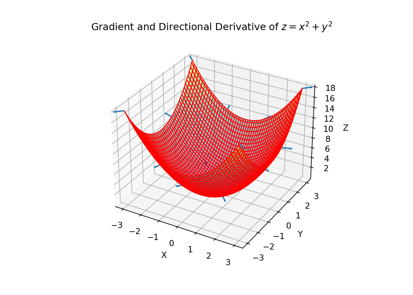

plt.show()

3.8.3.4 Normality of the Gradient

The gradient vector at a given point on a surface is normal (perpendicular) to the surface at that point. This means that the gradient vector points in a direction orthogonal to the tangent plane of the surface. This property is crucial in various applications:

• Optimization: The normality of the gradient helps in determining the direction of steepest ascent or descent, which is used in gradient-based optimization methods.
• Surface Normals: In computer graphics, the normal vector (which is the gradient vector) is used for shading and rendering, giving a realistic appearance to surfaces by simulating how light interacts with them.
• Physics: In physical simulations, the normal vector is used to calculate forces, collisions, and other interactions between objects.

For a function \(z = f(x, y)\), the gradient \(\nabla f\) at any point \((x, y)\) gives a vector that is perpendicular to the level curve passing through that point. This perpendicularity can be used to define tangent planes and normal lines, which are essential in differential geometry and related fields. One significant application of the gradient is in finding directional derivatives. The directional derivative of a function \(f(x, y)\) at a point \((x_0, y_0)\) in the direction of a unit vector \(\mathbf{u} = \langle a, b \rangle\) is given by the dot product of the gradient and the unit vector. This concept and its applications are explained in the next section.

3.8.4 Directional Derivatives in the Plane

Building upon our understanding of partial derivatives and the chain rule, we introduce the concept of directional derivatives. A directional derivative measures the rate at which a function changes as we move in a specific direction from a given point. This concept is particularly useful in fields like computer graphics and machine learning, where understanding how a function behaves in different directions is crucial.

Definition: Given a function \(f(x,y)\) and a direction vector \(\mathbf{u} = \langle a, b \rangle\), the directional derivative of \(f\) in the direction of \(\mathbf{u}\) at the point \((x_0, y_0)\) is defined as:

\[ D_{\mathbf{u}} f(x_0, y_0) = \lim_{h \to 0} \frac{f(x_0 + ha, y_0 + hb) - f(x_0, y_0)}{h} \]

This can be computed using the gradient of \(f\):

\[ D_{\mathbf{u}} f(x_0, y_0) = \nabla f(x_0, y_0) \cdot \mathbf{u} \]

where the gradient \(\nabla f(x, y)\) is the vector of partial derivatives:

\[ \nabla f(x, y) = \left\langle \frac{\partial f}{\partial x}, \frac{\partial f}{\partial y} \right\rangle \]

The directional derivative can then be expressed as:

\[ D_{\mathbf{u}} f(x_0, y_0) = \left( \frac{\partial f}{\partial x} \bigg|_{(x_0, y_0)}, \frac{\partial f}{\partial y} \bigg|_{(x_0, y_0)} \right) \cdot \langle a, b \rangle \]

Example 1: Directional Derivative of \(z = x^2 + y^2\)

Consider the function \(z = x^2 + y^2\). Let’s find the directional derivative at the point \((1, 1)\) in the direction of the vector \(\mathbf{u} = \langle 3, 4 \rangle\).

1. Compute the gradient: \[ \nabla f(x, y) = \left\langle \frac{\partial z}{\partial x}, \frac{\partial z}{\partial y} \right\rangle = \left\langle 2x, 2y \right\rangle \] At \((1, 1)\): \[ \nabla f(1, 1) = \left\langle 2 \cdot 1, 2 \cdot 1 \right\rangle = \langle 2, 2 \rangle \]

2. Normalize the direction vector: \[ \mathbf{u} = \langle 3, 4 \rangle \quad \text{with magnitude} \quad |\mathbf{u}| = \sqrt{3^2 + 4^2} = 5 \] \[ \mathbf{u} = \left\langle \frac{3}{5}, \frac{4}{5} \right\rangle = \left\langle 0.6, 0.8 \right\rangle \]

3. Calculate the directional derivative: \[ D_{\mathbf{u}} f(1, 1) = \nabla f(1, 1) \cdot \mathbf{u} = \langle 2, 2 \rangle \cdot \langle 0.6, 0.8 \rangle = 2 \cdot 0.6 + 2 \cdot 0.8 = 1.2 + 1.6 = 2.8 \]

Thus, the directional derivative of \(z = x^2 + y^2\) at the point \((1, 1)\) in the direction of \(\mathbf{u} = \langle 3, 4 \rangle\) is 2.8.

Visualization

The plot below shows the function \(z = x^2 + y^2\), the gradient vectors at several points, and the specific directional derivative at \((1, 1)\) in the direction of \(\mathbf{u} = \langle 3, 4 \rangle\).

import numpy as np
import matplotlib.pyplot as plt
from mpl_toolkits.mplot3d import Axes3D

# Define the function
def f(x, y):
    return x**2 + y**2

# Define the gradient
def grad_f(x, y):
    return np.array([2*x, 2*y])

# Define the points and the direction vector
x0, y0 = 1, 1
u = np.array([3, 4])
u = u / np.linalg.norm(u)  # Normalize the direction vector

# Create the grid for plotting
x = np.linspace(-3, 3, 100)
y = np.linspace(-3, 3, 100)
x, y = np.meshgrid(x, y)
z = f(x, y)

# Plot the surface
fig = plt.figure()
ax = fig.add_subplot(111, projection='3d')
ax.plot_surface(x, y, z, alpha=0.5, rstride=100, cstride=100)

## <mpl_toolkits.mplot3d.art3d.Poly3DCollection object at 0x0000029F56AB3C70>

# Plot the gradient vectors
for i in range(-3, 4, 2):
    for j in range(-3, 4, 2):
        ax.quiver(i, j, f(i, j), *grad_f(i, j), 0, length=0.5, normalize=True)

## <mpl_toolkits.mplot3d.art3d.Line3DCollection object at 0x0000029F5702BFD0>
## <mpl_toolkits.mplot3d.art3d.Line3DCollection object at 0x0000029F58D5D700>
## <mpl_toolkits.mplot3d.art3d.Line3DCollection object at 0x0000029F58D5D550>
## <mpl_toolkits.mplot3d.art3d.Line3DCollection object at 0x0000029F58D5D5B0>
## <mpl_toolkits.mplot3d.art3d.Line3DCollection object at 0x0000029F58D5DAF0>
## <mpl_toolkits.mplot3d.art3d.Line3DCollection object at 0x0000029F5701E8E0>
## <mpl_toolkits.mplot3d.art3d.Line3DCollection object at 0x0000029F5701E3D0>
## <mpl_toolkits.mplot3d.art3d.Line3DCollection object at 0x0000029F56AB33A0>
## <mpl_toolkits.mplot3d.art3d.Line3DCollection object at 0x0000029F56AB38B0>
## <mpl_toolkits.mplot3d.art3d.Line3DCollection object at 0x0000029F56A789A0>
## <mpl_toolkits.mplot3d.art3d.Line3DCollection object at 0x0000029F58EACA90>
## <mpl_toolkits.mplot3d.art3d.Line3DCollection object at 0x0000029F58EAC4F0>
## <mpl_toolkits.mplot3d.art3d.Line3DCollection object at 0x0000029F58EAC1C0>
## <mpl_toolkits.mplot3d.art3d.Line3DCollection object at 0x0000029F56D7A670>
## <mpl_toolkits.mplot3d.art3d.Line3DCollection object at 0x0000029F58F89F70>
## <mpl_toolkits.mplot3d.art3d.Line3DCollection object at 0x0000029F58F89D60>

# Plot the specific point and directional derivative
ax.quiver(x0, y0, f(x0, y0), *grad_f(x0, y0), 0, color='r', length=0.5, normalize=True)

## <mpl_toolkits.mplot3d.art3d.Line3DCollection object at 0x0000029F56A416D0>

ax.quiver(x0, y0, f(x0, y0), *(u * 2.8), 0, color='g', length=0.5, normalize=True)

## <mpl_toolkits.mplot3d.art3d.Line3DCollection object at 0x0000029F58F89490>

ax.set_xlabel('X')

## Text(0.5, 0, 'X')

ax.set_ylabel('Y')

## Text(0.5, 0.5, 'Y')

ax.set_zlabel('Z')

## Text(0.5, 0, 'Z')

ax.set_title('Directional Derivative of $z = x^2 + y^2$')

## Text(0.5, 0.92, 'Directional Derivative of $z = x^2 + y^2$')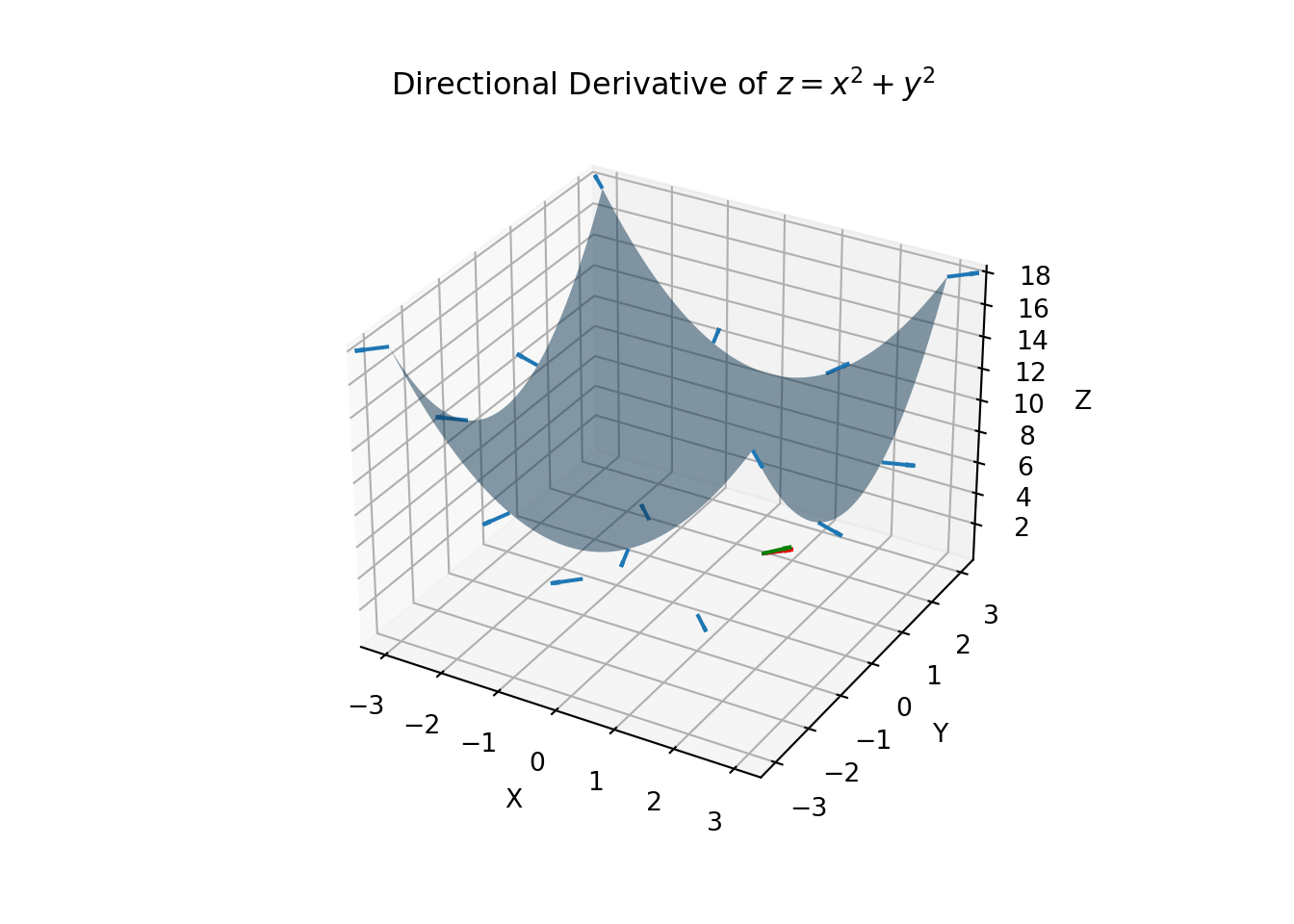

plt.show()

3.8.4.1 Practice Problems

1. Problem 1: Find the directional derivative of \(f(x, y) = x^2 + y^2\) at the point \((1, 2)\) in the direction of the vector \(\mathbf{v} = \langle 3, 4 \rangle\).

   Solution: \[ \nabla f = \langle 2x, 2y \rangle \] \[ \nabla f(1, 2) = \langle 2 \cdot 1, 2 \cdot 2 \rangle = \langle 2, 4 \rangle \] Normalize \(\mathbf{v}\): \[ \| \mathbf{v} \| = \sqrt{3^2 + 4^2} = 5 \] \[ \hat{\mathbf{v}} = \frac{1}{5} \langle 3, 4 \rangle = \langle \frac{3}{5}, \frac{4}{5} \rangle \] Directional derivative: \[ D_{\mathbf{v}} f = \nabla f \cdot \hat{\mathbf{v}} = \langle 2, 4 \rangle \cdot \langle \frac{3}{5}, \frac{4}{5} \rangle = \frac{6}{5} + \frac{16}{5} = \frac{22}{5} \] Interpretation: This value represents the rate of change of \(f\) in the direction of \(\mathbf{v}\) at the point \((1, 2)\).

2. Problem 2: Calculate the directional derivative of \(f(x, y) = \sin(xy)\) at the point \((0, \pi)\) in the direction of \(\mathbf{v} = \langle 1, 1 \rangle\).

   Solution: \[ \nabla f = \langle y \cos(xy), x \cos(xy) \rangle \] \[ \nabla f(0, \pi) = \langle \pi \cos(0), 0 \cdot \cos(0) \rangle = \langle \pi, 0 \rangle \] Normalize \(\mathbf{v}\): \[ \| \mathbf{v} \| = \sqrt{1^2 + 1^2} = \sqrt{2} \] \[ \hat{\mathbf{v}} = \frac{1}{\sqrt{2}} \langle 1, 1 \rangle = \langle \frac{1}{\sqrt{2}}, \frac{1}{\sqrt{2}} \rangle \] Directional derivative: \[ D_{\mathbf{v}} f = \nabla f \cdot \hat{\mathbf{v}} = \langle \pi, 0 \rangle \cdot \langle \frac{1}{\sqrt{2}}, \frac{1}{\sqrt{2}} \rangle = \frac{\pi}{\sqrt{2}} \] Interpretation: This value shows how \(f\) changes as we move from \((0, \pi)\) in the direction of \(\mathbf{v}\).

3. Problem 3: Find the directional derivative of \(f(x, y) = e^{x+y}\) at \((1, 0)\) in the direction of \(\mathbf{v} = \langle -1, 2 \rangle\).

   Solution: \[ \nabla f = \langle e^{x+y}, e^{x+y} \rangle \] \[ \nabla f(1, 0) = \langle e^1, e^1 \rangle = \langle e, e \rangle \] Normalize \(\mathbf{v}\): \[ \| \mathbf{v} \| = \sqrt{(-1)^2 + 2^2} = \sqrt{5} \] \[ \hat{\mathbf{v}} = \frac{1}{\sqrt{5}} \langle -1, 2 \rangle = \langle -\frac{1}{\sqrt{5}}, \frac{2}{\sqrt{5}} \rangle \] Directional derivative: \[ D_{\mathbf{v}} f = \nabla f \cdot \hat{\mathbf{v}} = \langle e, e \rangle \cdot \langle -\frac{1}{\sqrt{5}}, \frac{2}{\sqrt{5}} \rangle = -\frac{e}{\sqrt{5}} + \frac{2e}{\sqrt{5}} = \frac{e}{\sqrt{5}} \] Interpretation: This value gives the rate at which \(f\) changes in the direction of \(\mathbf{v}\) starting from \((1, 0)\).

4. Problem 4: Compute the directional derivative of \(f(x, y) = \ln(x^2 + y^2)\) at \((2, 1)\) in the direction of \(\mathbf{v} = \langle 4, -3 \rangle\).

   Solution: \[ \nabla f = \langle \frac{2x}{x^2 + y^2}, \frac{2y}{x^2 + y^2} \rangle \] \[ \nabla f(2, 1) = \langle \frac{4}{5}, \frac{2}{5} \rangle \] Normalize \(\mathbf{v}\): \[ \| \mathbf{v} \| = \sqrt{4^2 + (-3)^2} = 5 \] \[ \hat{\mathbf{v}} = \frac{1}{5} \langle 4, -3 \rangle = \langle \frac{4}{5}, -\frac{3}{5} \rangle \] Directional derivative: \[ D_{\mathbf{v}} f = \nabla f \cdot \hat{\mathbf{v}} = \langle \frac{4}{5}, \frac{2}{5} \rangle \cdot \langle \frac{4}{5}, -\frac{3}{5} \rangle = \frac{16}{25} - \frac{6}{25} = \frac{10}{25} = \frac{2}{5} \] Interpretation: This value indicates how fast \(f\) increases or decreases in the direction of \(\mathbf{v}\) at the point \((2, 1)\).

5. Problem 5: Determine the directional derivative of \(f(x, y) = x e^y\) at \((1, 1)\) in the direction of \(\mathbf{v} = \langle 2, -1 \rangle\).

   Solution: \[ \nabla f = \langle e^y, x e^y \rangle \] \[ \nabla f(1, 1) = \langle e^1, 1 \cdot e^1 \rangle = \langle e, e \rangle \] Normalize \(\mathbf{v}\): \[ \| \mathbf{v} \| = \sqrt{2^2 + (-1)^2} = \sqrt{5} \] \[ \hat{\mathbf{v}} = \frac{1}{\sqrt{5}} \langle 2, -1 \rangle = \langle \frac{2}{\sqrt{5}}, -\frac{1}{\sqrt{5}} \rangle \] Directional derivative: \[ D_{\mathbf{v}} f = \nabla f \cdot \hat{\mathbf{v}} = \langle e, e \rangle \cdot \langle \frac{2}{\sqrt{5}}, -\frac{1}{\sqrt{5}} \rangle = \frac{2e}{\sqrt{5}} - \frac{e}{\sqrt{5}} = \frac{e}{\sqrt{5}} \] Interpretation: This tells us the rate of change of \(f\) in the direction of \(\mathbf{v}\) at \((1, 1)\).

6. Problem 6: Find the directional derivative of \(f(x, y) = \cos(x) \sin(y)\) at \((\pi, \frac{\pi}{2})\) in the direction of \(\mathbf{v} = \langle 0, 1 \rangle\).

   Solution: \[ \nabla f = \langle -\sin(x) \sin(y), \cos(x) \cos(y) \rangle \] \[ \nabla f(\pi, \frac{\pi}{2}) = \langle -\sin(\pi) \sin(\frac{\pi}{2}), \cos(\pi) \cos(\frac{\pi}{2}) \rangle = \langle 0, 0 \rangle \] Normalize \(\mathbf{v}\): \[ \| \mathbf{v} \| = \sqrt{0^2 + 1^2} = 1 \] \[ \hat{\mathbf{v}} = \langle 0, 1 \rangle \] Directional derivative: \[ D_{\mathbf{v}} f = \nabla f \cdot \hat{\mathbf{v}} = \langle 0, 0 \rangle \cdot \langle 0, 1 \rangle = 0 \] Interpretation: Since the gradient is zero, the function does not change in the direction of \(\mathbf{v}\) at \((\pi, \frac{\pi}{2})\).

7. Problem 7: Compute the directional derivative of \(f(x, y) = x^2 - y^2\) at \((1, -1)\) in the direction of \(\mathbf{v} = \langle 1, 2 \rangle\).

   Solution: \[ \nabla f = \langle 2x, -2y \rangle \] \[ \nabla f(1, -1) = \langle 2 \cdot 1, -2 \cdot (-1) \rangle = \langle 2, 2 \rangle \] Normalize \(\mathbf{v}\): \[ \| \mathbf{v} \| = \sqrt{1^2 + 2^2} = \sqrt{5} \] \[ \hat{\mathbf{v}} = \frac{1}{\sqrt{5}} \langle 1, 2 \rangle = \langle \frac{1}{\sqrt{5}}, \frac{2}{\sqrt{5}} \rangle \] Directional derivative: \[ D_{\mathbf{v}} f = \nabla f \cdot \hat{\mathbf{v}} = \langle 2, 2 \rangle \cdot \langle \frac{1}{\sqrt{5}}, \frac{2}{\sqrt{5}} \rangle = \frac{2}{\sqrt{5}} + \frac{4}{\sqrt{5}} = \frac{6}{\sqrt{5}} \] Interpretation: This value gives the rate of change of \(f\) in the direction of \(\mathbf{v}\) at the point \((1, -1)\).

8. Problem 8: Find the directional derivative of \(f(x, y) = \sqrt{x^2 + y^2}\) at \((2, 3)\) in the direction of \(\mathbf{v} = \langle -3, 4 \rangle\).

   Solution: \[ \nabla f = \langle \frac{x}{\sqrt{x^2 + y^2}}, \frac{y}{\sqrt{x^2 + y^2}} \rangle \] \[ \nabla f(2, 3) = \langle \frac{2}{\sqrt{13}}, \frac{3}{\sqrt{13}} \rangle \] Normalize \(\mathbf{v}\): \[ \| \mathbf{v} \| = \sqrt{(-3)^2 + 4^2} = 5 \] \[ \hat{\mathbf{v}} = \frac{1}{5} \langle -3, 4 \rangle = \langle -\frac{3}{5}, \frac{4}{5} \rangle \] Directional derivative: \[ D_{\mathbf{v}} f = \nabla f \cdot \hat{\mathbf{v}} = \langle \frac{2}{\sqrt{13}}, \frac{3}{\sqrt{13}} \rangle \cdot \langle -\frac{3}{5}, \frac{4}{5} \rangle = -\frac{6}{5\sqrt{13}} + \frac{12}{5\sqrt{13}} = \frac{6}{5\sqrt{13}} \] Interpretation: This value indicates the rate of change of \(f\) in the direction of \(\mathbf{v}\) at \((2, 3)\).

9. Problem 9: Calculate the directional derivative of \(f(x, y) = \tan(xy)\) at \((1, 1)\) in the direction of \(\mathbf{v} = \langle 2, -1 \rangle\).

   Solution: \[ \nabla f = \langle y \sec^2(xy), x \sec^2(xy) \rangle \] \[ \nabla f(1, 1) = \langle 1 \cdot \sec^2(1), 1 \cdot \sec^2(1) \rangle = \langle \sec^2(1), \sec^2(1) \rangle \] Normalize \(\mathbf{v}\): \[ \| \mathbf{v} \| = \sqrt{2^2 + (-1)^2} = \sqrt{5} \] \[ \hat{\mathbf{v}} = \frac{1}{\sqrt{5}} \langle 2, -1 \rangle = \langle \frac{2}{\sqrt{5}}, -\frac{1}{\sqrt{5}} \rangle \] Directional derivative: \[ D_{\mathbf{v}} f = \nabla f \cdot \hat{\mathbf{v}} = \langle \sec^2(1), \sec^2(1) \rangle \cdot \langle \frac{2}{\sqrt{5}}, -\frac{1}{\sqrt{5}} \rangle = \frac{2 \sec^2(1)}{\sqrt{5}} - \frac{\sec^2(1)}{\sqrt{5}} = \frac{\sec^2(1)}{\sqrt{5}} \] Interpretation: This value tells how fast \(f\) changes in the direction of \(\mathbf{v}\) at \((1, 1)\).

10. Problem 10: Determine the directional derivative of \(f(x, y) = x^3 y - y^3 x\) at \((1, 2)\) in the direction of \(\mathbf{v} = \langle 1, 1 \rangle\).

    Solution: \[ \nabla f = \langle 3x^2 y - y^3, x^3 - 3y^2 x \rangle \] \[ \nabla f(1, 2) = \langle 3 \cdot 1^2 \cdot 2 - 2^3, 1^3 - 3 \cdot 2^2 \cdot 1 \rangle = \langle 6 - 8, 1 - 12 \rangle = \langle -2, -11 \rangle \] Normalize \(\mathbf{v}\): \[ \| \mathbf{v} \| = \sqrt{1^2 + 1^2} = \sqrt{2} \] \[ \hat{\mathbf{v}} = \frac{1}{\sqrt{2}} \langle 1, 1 \rangle = \langle \frac{1}{\sqrt{2}}, \frac{1}{\sqrt{2}} \rangle \] Directional derivative: \[ D_{\mathbf{v}} f = \nabla f \cdot \hat{\mathbf{v}} = \langle -2, -11 \rangle \cdot \langle \frac{1}{\sqrt{2}}, \frac{1}{\sqrt{2}} \rangle = \frac{-2}{\sqrt{2}} + \frac{-11}{\sqrt{2}} = \frac{-13}{\sqrt{2}} \] Interpretation: This value shows how \(f\) changes in the direction of \(\mathbf{v}\) at the point \((1, 2)\).

3.8.4.2 Application Problems

1. Application Problem 1: A company’s profit function is \(P(x, y) = x^2 y + xy^2\), where \(x\) represents units of product A and \(y\) represents units of product B. Find the rate of change of profit when \(x = 2\) and \(y = 3\) in the direction of increasing production of product B.

   Solution: \[ \nabla P = \langle 2xy + y^2, x^2 + 2xy \rangle \] \[ \nabla P(2, 3) = \langle 2 \cdot 2 \cdot 3 + 3^2, 2^2 + 2 \cdot 2 \cdot 3 \rangle = \langle 12 + 9, 4 + 12 \rangle = \langle 21, 16 \rangle \] Direction of increasing production of product B: \(\mathbf{v} = \langle 0, 1 \rangle\) \[ D_{\mathbf{v}} P = \nabla P \cdot \mathbf{v} = \langle 21, 16 \rangle \cdot \langle 0, 1 \rangle = 16 \] Interpretation: The profit increases by 16 units for each additional unit of product B produced, keeping \(x = 2\).

2. Application Problem 2: A temperature distribution in a metal plate is given by \(T(x, y) = 100 e^{-0.1(x^2 + y^2)}\). Compute the rate of temperature change at \((3, 4)\) in the direction of the vector \(\mathbf{v} = \langle 4, 3 \rangle\).

   Solution: \[ \nabla T = \langle -0.2 x e^{-0.1(x^2 + y^2)}, -0.2 y e^{-0.1(x^2 + y^2)} \rangle \] \[ \nabla T(3, 4) = \langle -0.2 \cdot 3 \cdot e^{-0.1(3^2 + 4^2)}, -0.2 \cdot 4 \cdot e^{-0.1(3^2 + 4^2)} \rangle = \langle -0.6 e^{-0.1 \cdot 25}, -0.8 e^{-0.1 \cdot 25} \rangle \] Normalize \(\mathbf{v}\): \[ \| \mathbf{v} \| = 5 \] \[ \hat{\mathbf{v}} = \frac{1}{5} \langle 4, 3 \rangle = \langle \frac{4}{5}, \frac{3}{5} \rangle \] Directional derivative: \[ D_{\mathbf{v}} T = \nabla T \cdot \hat{\mathbf{v}} = \langle -0.6 e^{-2.5}, -0.8 e^{-2.5} \rangle \cdot \langle \frac{4}{5}, \frac{3}{5} \rangle = -0.6 e^{-2.5} \cdot \frac{4}{5} - 0.8 e^{-2.5} \cdot \frac{3}{5} = -e^{-2.5} \] Interpretation: The temperature decreases by \(e^{-2.5}\) units per unit length in the direction of \(\mathbf{v}\) at \((3, 4)\).

3. Application Problem 3: The height of a hill at point \((x, y)\) is given by \(h(x, y) = 5 - x^2 - y^2\). Find the rate at which the height changes as you move from point \((1, 2)\) in the direction of \(\mathbf{v} = \langle 1, -1 \rangle\).

   Solution: \[ \nabla h = \langle -2x, -2y \rangle \] \[ \nabla h(1, 2) = \langle -2 \cdot 1, -2 \cdot 2 \rangle = \langle -2, -4 \rangle \] Normalize \(\mathbf{v}\): \[ \| \mathbf{v} \| = \sqrt{1^2 + (-1)^2} = \sqrt{2} \] \[ \hat{\mathbf{v}} = \frac{1}{\sqrt{2}} \langle 1, -1 \rangle = \langle \frac{1}{\sqrt{2}}, -\frac{1}{\sqrt{2}} \rangle \] Directional derivative: \[ D_{\mathbf{v}} h = \nabla h \cdot \hat{\mathbf{v}} = \langle -2, -4 \rangle \cdot \langle \frac{1}{\sqrt{2}}, -\frac{1}{\sqrt{2}} \rangle = -\frac{2}{\sqrt{2}} + \frac{4}{\sqrt{2}} = \sqrt{2} \] Interpretation: The height of the hill increases at a rate of \(\sqrt{2}\) units per unit length in the direction of \(\mathbf{v}\) at \((1, 2)\).

4. Application Problem 4: In a manufacturing process, the production rate function is \(P(x, y) = x^2 y - xy^2\). Determine the rate of change of production when \(x = 3\) and \(y = 2\) in the direction of \(\mathbf{v} = \langle -1, 1 \rangle\).

   Solution: \[ \nabla P = \langle 2xy - y^2, x^2 - 2xy \rangle \] \[ \nabla P(3, 2) = \langle 2 \cdot 3 \cdot 2 - 2^2, 3^2 - 2 \cdot 3 \cdot 2 \rangle = \langle 6, -6 \rangle \] Normalize \(\mathbf{v}\): \[ \| \mathbf{v} \| = \sqrt{(-1)^2 + 1^2} = \sqrt{2} \] \[ \hat{\mathbf{v}} = \frac{1}{\sqrt{2}} \langle -1, 1 \rangle = \langle -\frac{1}{\sqrt{2}}, \frac{1}{\sqrt{2}} \rangle \] Directional derivative: \[ D_{\mathbf{v}} P = \nabla P \cdot \hat{\mathbf{v}} = \langle 6, -6 \rangle \cdot \langle -\frac{1}{\sqrt{2}}, \frac{1}{\sqrt{2}} \rangle = -\frac{6}{\sqrt{2}} - \frac{6}{\sqrt{2}} = -6 \sqrt{2} \] Interpretation: The production rate decreases by \(6 \sqrt{2}\) units per unit length in the direction of \(\mathbf{v}\) at \((3, 2)\).

5. Application Problem 5: Consider a landscape with height \(h(x, y) = 10 - x^2 - 2y^2\). Find the rate at which the height changes at \((2, 1)\) in the direction of \(\mathbf{v} = \langle 2, -1 \rangle\).

   Solution: \[ \nabla h = \langle -2x, -4y \rangle \] \[ \nabla h(2, 1) = \langle -2 \cdot 2, -4 \cdot 1 \rangle = \langle -4, -4 \rangle \] Normalize \(\mathbf{v}\): \[ \| \mathbf{v} \| = \sqrt{2^2 + (-1)^2} = \sqrt{5} \] \[ \hat{\mathbf{v}} = \frac{1}{\sqrt{5}} \langle 2, -1 \rangle = \langle \frac{2}{\sqrt{5}}, -\frac{1}{\sqrt{5}} \rangle \] Directional derivative: \[ D_{\mathbf{v}} h = \nabla h \cdot \hat{\mathbf{v}} = \langle -4, -4 \rangle \cdot \langle \frac{2}{\sqrt{5}}, -\frac{1}{\sqrt{5}} \rangle = -\frac{8}{\sqrt{5}} + \frac{4}{\sqrt{5}} = -\frac{4}{\sqrt{5}} \] Interpretation: The height decreases by \(\frac{4}{\sqrt{5}}\) units per unit length in the direction of \(\mathbf{v}\) at \((2, 1)\).

Application Problem 6: In an optimization problem for resource allocation \(A(x, y) = x^2 y + xy^2\), where \(x\) and \(y\) represent quantities of two resources, find the rate of change of \(A\) at \((3, 4)\) in the direction of \(\mathbf{v} = \langle 1, 2 \rangle\).

Solution:

\[ \nabla A = \langle 2xy + y^2, x^2 + 2xy \rangle \]

\[ \nabla A(3, 4) = \langle 2 \cdot 3 \cdot 4 + 4^2, 3^2 + 2 \cdot 3 \cdot 4 \rangle = \langle 24 + 16, 9 + 24 \rangle = \langle 40, 33 \rangle \]

Normalize \(\mathbf{v}\):

\[ \| \mathbf{v} \| = \sqrt{1^2 + 2^2} = \sqrt{5} \]

\[ \hat{\mathbf{v}} = \frac{1}{\sqrt{5}} \langle 1, 2 \rangle = \langle \frac{1}{\sqrt{5}}, \frac{2}{\sqrt{5}} \rangle \]

Directional derivative:

\[ D_{\mathbf{v}} A = \nabla A \cdot \hat{\mathbf{v}} = \langle 40, 33 \rangle \cdot \langle \frac{1}{\sqrt{5}}, \frac{2}{\sqrt{5}} \rangle = \frac{40}{\sqrt{5}} + \frac{66}{\sqrt{5}} = \frac{106}{\sqrt{5}} \]

Interpretation: The resource allocation function increases by \(\frac{106}{\sqrt{5}}\) units per unit length in the direction of the vector \(\mathbf{v}\), showing increased efficiency in resource utilization.

---

Application Problem 7: In a function describing error in machine learning \(E(x, y) = \exp(x) - y^2\), where \(x\) is the complexity and \(y\) is the regularization parameter, find the rate of change of error at \((0, 1)\) in the direction of \(\mathbf{v} = \langle 1, 0 \rangle\).

Solution:

\[ \nabla E = \langle \exp(x), -2y \rangle \]

\[ \nabla E(0, 1) = \langle \exp(0), -2 \cdot 1 \rangle = \langle 1, -2 \rangle \]

Normalize \(\mathbf{v}\):

\[ \| \mathbf{v} \| = \sqrt{1^2 + 0^2} = 1 \]

\[ \hat{\mathbf{v}} = \langle 1, 0 \rangle \]

Directional derivative:

\[ D_{\mathbf{v}} E = \nabla E \cdot \hat{\mathbf{v}} = \langle 1, -2 \rangle \cdot \langle 1, 0 \rangle = 1 \]

Interpretation: The error in the machine learning model increases by 1 unit per unit length in the direction of increasing model complexity.

---

Application Problem 8: For a performance function \(P(x, y) = x^2 - y^2\), where \(x\) and \(y\) are parameters affecting performance, compute the rate of change at \((2, -1)\) in the direction of \(\mathbf{v} = \langle -2, 3 \rangle\).

Solution:

\[ \nabla P = \langle 2x, -2y \rangle \]

\[ \nabla P(2, -1) = \langle 2 \cdot 2, -2 \cdot (-1) \rangle = \langle 4, 2 \rangle \]

Normalize \(\mathbf{v}\):

\[ \| \mathbf{v} \| = \sqrt{(-2)^2 + 3^2} = \sqrt{13} \]

\[ \hat{\mathbf{v}} = \frac{1}{\sqrt{13}} \langle -2, 3 \rangle = \langle -\frac{2}{\sqrt{13}}, \frac{3}{\sqrt{13}} \rangle \]

Directional derivative:

\[ D_{\mathbf{v}} P = \nabla P \cdot \hat{\mathbf{v}} = \langle 4, 2 \rangle \cdot \langle -\frac{2}{\sqrt{13}}, \frac{3}{\sqrt{13}} \rangle = -\frac{8}{\sqrt{13}} + \frac{6}{\sqrt{13}} = -\frac{2}{\sqrt{13}} \]

Interpretation: The performance function decreases by \(\frac{2}{\sqrt{13}}\) units per unit length in the direction of the vector \(\mathbf{v}\), indicating a reduction in performance as the parameters change.

---

Application Problem 9: In a simulation function \(S(x, y) = x \cdot \ln(y)\), where \(x\) and \(y\) represent parameters of a simulation, find the rate of change at \((2, e)\) in the direction of \(\mathbf{v} = \langle -1, 2 \rangle\).

Solution:

\[ \nabla S = \langle \ln(y), \frac{x}{y} \rangle \]

\[ \nabla S(2, e) = \langle \ln(e), \frac{2}{e} \rangle = \langle 1, \frac{2}{e} \rangle \]

Normalize \(\mathbf{v}\):

\[ \| \mathbf{v} \| = \sqrt{(-1)^2 + 2^2} = \sqrt{5} \]

\[ \hat{\mathbf{v}} = \frac{1}{\sqrt{5}} \langle -1, 2 \rangle = \langle -\frac{1}{\sqrt{5}}, \frac{2}{\sqrt{5}} \rangle \]

Directional derivative:

\[ D_{\mathbf{v}} S = \nabla S \cdot \hat{\mathbf{v}} = \langle 1, \frac{2}{e} \rangle \cdot \langle -\frac{1}{\sqrt{5}}, \frac{2}{\sqrt{5}} \rangle = -\frac{1}{\sqrt{5}} + \frac{4}{e \sqrt{5}} = \frac{4 - e}{e \sqrt{5}} \]

Interpretation: The simulation function changes at a rate of \(\frac{4 - e}{e \sqrt{5}}\) units per unit length in the direction of the vector \(\mathbf{v}\), reflecting how the simulation parameters affect the output.

---

Application Problem 10: For a loss function \(L(x, y) = e^{x+y}\), where \(x\) and \(y\) are model parameters, find the rate of change at \((0, 0)\) in the direction of \(\mathbf{v} = \langle 3, -4 \rangle\).

Solution:

\[ \nabla L = \langle e^{x+y}, e^{x+y} \rangle \]

\[ \nabla L(0, 0) = \langle e^{0+0}, e^{0+0} \rangle = \langle 1, 1 \rangle \]

Normalize \(\mathbf{v}\):

\[ \| \mathbf{v} \| = \sqrt{3^2 + (-4)^2} = 5 \]

\[ \hat{\mathbf{v}} = \frac{1}{5} \langle 3, -4 \rangle = \langle \frac{3}{5}, -\frac{4}{5} \rangle \]

Directional derivative:

\[ D_{\mathbf{v}} L = \nabla L \cdot \hat{\mathbf{v}} = \langle 1, 1 \rangle \cdot \langle \frac{3}{5}, -\frac{4}{5} \rangle = \frac{3}{5} - \frac{4}{5} = -\frac{1}{5} \]

Interpretation: The loss function decreases by \(\frac{1}{5}\) units per unit length in the direction of the vector \(\mathbf{v}\), showing a reduction in the model loss as the parameters change accordingly.

---

3.8.4.3 Properties of the Directional Derivative

The directional derivative of a function provides information about the rate at which the function changes as one moves in a specified direction. Here are some important properties of the directional derivative:

1. Linearity with Respect to the Direction Vector: The directional derivative is linear with respect to the direction vector. If \(\mathbf{v}_1\) and \(\mathbf{v}_2\) are two direction vectors, and \(a\) and \(b\) are scalars, then the directional derivative in the direction \(a \mathbf{v}_1 + b \mathbf{v}_2\) is given by: \[ D_{a \mathbf{v}_1 + b \mathbf{v}_2} f = a D_{\mathbf{v}_1} f + b D_{\mathbf{v}_2} f \]

2. Normalization of the Direction Vector: The directional derivative is calculated in the direction of a unit vector. If \(\mathbf{v}\) is any direction vector, the directional derivative in the direction \(\mathbf{v}\) can be expressed in terms of the unit vector \(\hat{\mathbf{v}} = \frac{\mathbf{v}}{\|\mathbf{v}\|}\): \[ D_{\mathbf{v}} f = \nabla f \cdot \hat{\mathbf{v}} \]

3. Directional Derivative as a Gradient Projection: The directional derivative in the direction of a unit vector \(\hat{\mathbf{v}}\) is the projection of the gradient vector \(\nabla f\) onto \(\hat{\mathbf{v}}\). Thus: \[ D_{\mathbf{v}} f = \nabla f \cdot \hat{\mathbf{v}} \]

4. Directional Derivative and Gradient Relationship: The directional derivative in the direction of \(\mathbf{v}\) can be computed using the gradient of the function as: \[ D_{\mathbf{v}} f = \nabla f \cdot \frac{\mathbf{v}}{\|\mathbf{v}\|} \] where \(\nabla f\) is the gradient of \(f\) and \(\frac{\mathbf{v}}{\|\mathbf{v}\|}\) is the unit vector in the direction of \(\mathbf{v}\).

5. Directional Derivative in Orthogonal Directions: If \(\mathbf{v}_1\) and \(\mathbf{v}_2\) are orthogonal vectors, then: \[ D_{\mathbf{v}_1 + \mathbf{v}_2} f = D_{\mathbf{v}_1} f + D_{\mathbf{v}_2} f \] This property follows from the linearity of the directional derivative.

6. Directional Derivative at a Point: The directional derivative of \(f\) at a point \(\mathbf{p}\) in the direction of a vector \(\mathbf{v}\) describes the rate of change of \(f\) at \(\mathbf{p}\) in that direction. Specifically, if \(f\) is differentiable at \(\mathbf{p}\), then: \[ D_{\mathbf{v}} f (\mathbf{p}) = \nabla f (\mathbf{p}) \cdot \frac{\mathbf{v}}{\|\mathbf{v}\|} \]

3.8.5 Relative Extrema: From Univariate to Multivariate Functions

In calculus, finding relative extrema (local maxima and minima) is essential for understanding the behavior of functions. While in univariate calculus we use the first and second derivatives to find and classify relative extrema, the process is extended to multivariate functions in a similar manner but with additional complexity. For a function \(f(x)\) of a single variable, finding relative extrema involves the following steps:

1. Finding Critical Points:
   • Solve \(f'(x) = 0\) to determine points where the derivative (slope) is zero.
2. Classifying Critical Points:
   • Use the second derivative test:
     • If \(f''(x) > 0\) at a critical point, it indicates a local minimum.
     • If \(f''(x) < 0\), it indicates a local maximum.
     • If \(f''(x) = 0\), the test is inconclusive, and further analysis is needed.

Transition to Multivariate Functions

For functions of two variables \(f(x, y)\), the process to find and classify relative extrema is more complex but follows a similar idea:

1. Finding Critical Points:
   • Solve the system of equations given by the first partial derivatives: \[ f_x = 0 \quad \text{and} \quad f_y = 0 \]
2. Classifying Critical Points:

   • Use the Hessian matrix to determine the nature of the critical points. The Hessian matrix \(H\) is defined as: \[ H = \begin{pmatrix} f_{xx} & f_{xy} \\ f_{xy} & f_{yy} \end{pmatrix} \] where:

     • \(f_{xx} = \frac{\partial^2 f}{\partial x^2}\)
     • \(f_{yy} = \frac{\partial^2 f}{\partial y^2}\)
     • \(f_{xy} = \frac{\partial^2 f}{\partial x \partial y}\)

   • The determinant of the Hessian matrix, \(D\), is calculated as: \[ D = f_{xx} f_{yy} - (f_{xy})^2 \]

   • The nature of the critical point is determined as follows:

     • Local Minimum: If \(D > 0\) and \(f_{xx} > 0\).
     • Local Maximum: If \(D > 0\) and \(f_{xx} < 0\).
     • Saddle Point: If \(D < 0\).
     • Inconclusive: If \(D = 0\).
3. Summary Table

To classify the nature of a critical point, use the following table:

Sl. No	Critical Points	\(r = \frac{\partial^2 f}{\partial x^2}\)	\(t = \frac{\partial^2 f}{\partial y^2}\)	\(s = \frac{\partial^2 f}{\partial x \partial y}\)	\(D = rt - s^2\)	Nature	Extremum
1	\((x_0, y_0)\)	\(f_{xx}(x_0, y_0)\)	\(f_{yy}(x_0, y_0)\)	\(f_{xy}(x_0, y_0)\)	\(f_{xx} f_{yy} - (f_{xy})^2\)	To be determined based on \(D\)	To be determined

Example:

Find and classify the critical points of the function \(f(x, y) = x^3 - 3x y^2\).

Solution:

1. Find Critical Points:

   Compute the first partial derivatives:

   \[ f_x = \frac{\partial f}{\partial x} = 3x^2 - 3y^2 \] \[ f_y = \frac{\partial f}{\partial y} = -6xy \]

   Set these equal to zero:

   \[ 3x^2 - 3y^2 = 0 \] \[ -6xy = 0 \]

   Solving these equations, we find the critical point at \((0, 0)\).

2. Classify the Critical Point:

   Compute the second partial derivatives:

   \[ f_{xx} = \frac{\partial^2 f}{\partial x^2} = 6x \] \[ f_{yy} = \frac{\partial^2 f}{\partial y^2} = -6x \] \[ f_{xy} = \frac{\partial^2 f}{\partial x \partial y} = -6y \]

   Evaluate these at \((0, 0)\):

   \[ f_{xx}(0, 0) = 0 \] \[ f_{yy}(0, 0) = 0 \] \[ f_{xy}(0, 0) = 0 \]

   Compute the determinant \(D\):

   \[ D = f_{xx}(0, 0) \cdot f_{yy}(0, 0) - (f_{xy}(0, 0))^2 = 0 \cdot 0 - 0^2 = 0 \]

   Since \(D = 0\), the test is inconclusive. Further analysis shows that the point \((0, 0)\) is a saddle point.

Summary Table for Example

Sl. No	Critical Points	\(r = f_{xx}\)	\(t = f_{yy}\)	\(s = f_{xy}\)	\(D = rt - s^2\)	Nature	Extremum
1	\((0, 0)\)	\(0\)	\(0\)	\(0\)	\(0\)	Inconclusive (Further Analysis Needed)	None

---

Visualization

import numpy as np
import matplotlib.pyplot as plt
from mpl_toolkits.mplot3d import Axes3D

# Define the function
def f(x, y):
    return x**3 - 3*x*y**2

# Define the gradient and Hessian matrix components
def gradient(x, y):
    fx = 3*x**2 - 3*y**2
    fy = -6*x*y
    return fx, fy

def hessian(x, y):
    fxx = 6*x
    fyy = -6*x
    fxy = -6*y
    return fxx, fyy, fxy

# Define the grid
x = np.linspace(-2, 2, 400)
y = np.linspace(-2, 2, 400)
X, Y = np.meshgrid(x, y)
Z = f(X, Y)

# Compute the Hessian matrix at the critical point (0, 0)
x0, y0 = 0, 0
fxx, fyy, fxy = hessian(x0, y0)
D = fxx * fyy - fxy**2

# Create the figure and axis
fig = plt.figure(figsize=(12, 6))

# 3D Surface Plot
ax1 = fig.add_subplot(121, projection='3d')
ax1.plot_surface(X, Y, Z, cmap='viridis', alpha=0.8)

## <mpl_toolkits.mplot3d.art3d.Poly3DCollection object at 0x0000029F569901C0>

ax1.scatter(x0, y0, f(x0, y0), color='r', s=50)  # Critical point

## <mpl_toolkits.mplot3d.art3d.Path3DCollection object at 0x0000029F56A5E4C0>

ax1.set_title('3D Surface Plot')

## Text(0.5, 0.92, '3D Surface Plot')

ax1.set_xlabel('x')

## Text(0.5, 0, 'x')

ax1.set_ylabel('y')

## Text(0.5, 0.5, 'y')

ax1.set_zlabel('f(x, y)')

## Text(0.5, 0, 'f(x, y)')

# Contour Plot
ax2 = fig.add_subplot(122)
contour = ax2.contour(X, Y, Z, levels=20, cmap='viridis')
ax2.scatter(x0, y0, color='r', s=50)  # Critical point

## <matplotlib.collections.PathCollection object at 0x0000029F573A1610>

ax2.set_title('Contour Plot')

## Text(0.5, 1.0, 'Contour Plot')

ax2.set_xlabel('x')

## Text(0.5, 0, 'x')

ax2.set_ylabel('y')

## Text(0, 0.5, 'y')

fig.colorbar(contour, ax=ax2)

## <matplotlib.colorbar.Colorbar object at 0x0000029F56B34520>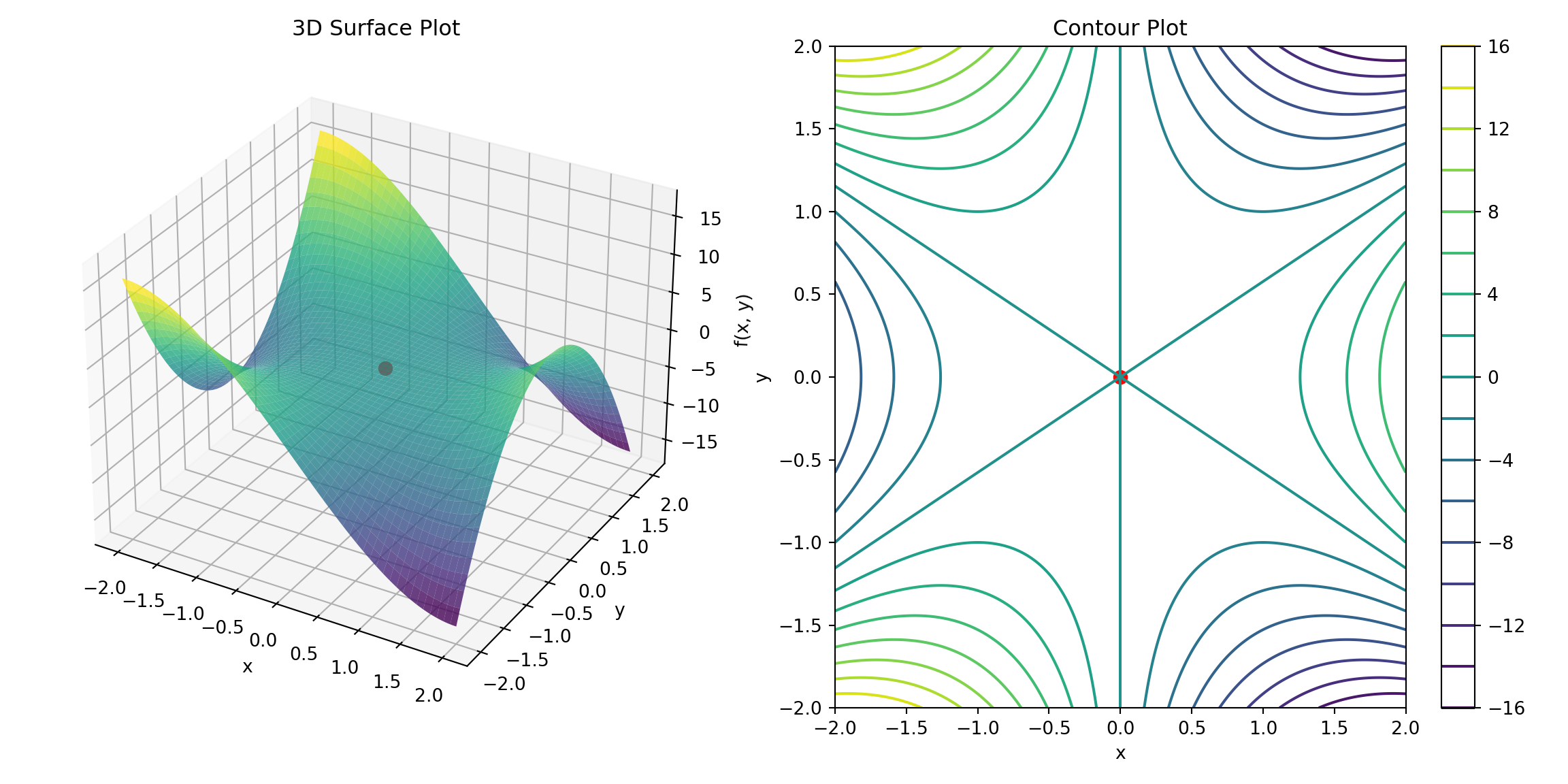

# Show the plots
plt.tight_layout()
plt.show()

# Print out the classification based on Hessian determinant
#print("Hessian Matrix at (0, 0):")
#print(f"fxx = {fxx}, fyy = {fyy}, fxy = {fxy}")
#print(f"Determinant D = {D}")

#if D > 0:
#    if fxx > 0:
#        print("Local Minimum")
#    else:
#        print("Local Maximum")
#elif D < 0:
#    print("Saddle Point")
#else:
#    print("Inconclusive (Further Analysis Needed)")

Problem 1: Find the relative extrema of \(f(x, y) = x^3 - 3x y^2\).

Solution:

1. Compute the partial derivatives: \[ \frac{\partial f}{\partial x} = 3x^2 - 3y^2 \] \[ \frac{\partial f}{\partial y} = -6xy \]

2. Set the partial derivatives to zero: \[ 3x^2 - 3y^2 = 0 \quad \text{and} \quad -6xy = 0 \] Solving these gives \(x = 0\) or \(y = 0\). For \(x = 0\), \(y = 0\) is a critical point. For \(y = 0\), \(x^2 = y^2\), so \(x = \pm y\).

3. Compute the Hessian matrix: \[ H = \begin{bmatrix} 6x & -6y \\ -6y & -6x \end{bmatrix} \]

4. Compute the determinant \(D\): \[ D = (6x)(-6x) - (-6y)^2 = -36x^2 - 36y^2 \] At \((0, 0)\): \[ D = -36 \cdot 0 - 36 \cdot 0 = 0 \]

5. Classify the critical point:

   • Since \(D = 0\), the test is inconclusive. Further analysis shows that \((0, 0)\) is a saddle point.

Summary Table:

Sl. No	Critical Points	r	D = rt - s²	Nature	Extremum
1	(0, 0)	0	0	Saddle Point	N/A

---

Problem 2: Find the relative extrema of \(f(x, y) = x^2 + y^2 - 2x - 2y\).

Solution:

1. Compute the partial derivatives: \[ \frac{\partial f}{\partial x} = 2x - 2 \] \[ \frac{\partial f}{\partial y} = 2y - 2 \]

2. Set the partial derivatives to zero: \[ 2x - 2 = 0 \quad \text{and} \quad 2y - 2 = 0 \] Solving these gives \(x = 1\) and \(y = 1\).

3. Compute the Hessian matrix: \[ H = \begin{bmatrix} 2 & 0 \\ 0 & 2 \end{bmatrix} \]

4. Compute the determinant \(D\): \[ D = (2)(2) - 0^2 = 4 \] At \((1, 1)\): \[ D = 4 \]

5. Classify the critical point:

   • Since \(D > 0\) and \(f_{xx} > 0\), it is a local minimum.

Summary Table:

Sl. No	Critical Points	r	D = rt - s²	Nature	Extremum
1	(1, 1)	2	4	Local Min	Minimum

---

Problem 3: Determine the relative extrema of \(f(x, y) = x^4 + y^4 - 4x^2 - 4y^2\).

Solution:

1. Compute the partial derivatives: \[ \frac{\partial f}{\partial x} = 4x^3 - 8x \] \[ \frac{\partial f}{\partial y} = 4y^3 - 8y \]

2. Set the partial derivatives to zero: \[ 4x^3 - 8x = 0 \quad \text{and} \quad 4y^3 - 8y = 0 \] Solving these gives \(x = 0, \pm 2\) and \(y = 0, \pm 2\).

3. Compute the Hessian matrix: \[ H = \begin{bmatrix} 12x^2 - 8 & 0 \\ 0 & 12y^2 - 8 \end{bmatrix} \]

4. Compute the determinant \(D\): \[ D = (12x^2 - 8)(12y^2 - 8) - 0^2 \] At \((0, 0)\): \[ D = (-8)(-8) = 64 \]

5. Classify the critical point:

   • Since \(D > 0\) and \(f_{xx} > 0\), it is a local minimum.

Summary Table:

Sl. No	Critical Points	r	D = rt - s²	Nature	Extremum
1	(0, 0)	-8	64	Local Min	Minimum
2	(2, 2)	16	64	Local Min	Minimum
3	(-2, -2)	16	64	Local Min	Minimum
4	(2, -2)	16	64	Local Min	Minimum
5	(-2, 2)	16	64	Local Min	Minimum

---

Problem 4: Find the relative extrema of \(f(x, y) = e^{x+y}\).

Solution:

1. Compute the partial derivatives: \[ \frac{\partial f}{\partial x} = e^{x+y} \] \[ \frac{\partial f}{\partial y} = e^{x+y} \]

2. Set the partial derivatives to zero: \[ e^{x+y} = 0 \] There are no solutions because \(e^{x+y}\) is never zero.

3. No critical points exist for this function.

Summary Table:

Sl. No	Critical Points	r	D = rt - s²	Nature	Extremum
1	None	-	-	N/A	N/A

---

Problem 5: Determine the relative extrema of \(f(x, y) = \frac{x^2 y}{x^2 + y^2}\) for \((x, y) \neq (0, 0)\).

Solution:

1. Compute the partial derivatives: \[ \frac{\partial f}{\partial x} = \frac{2xy^3}{(x^2 + y^2)^2} \] \[ \frac{\partial f}{\partial y} = \frac{x^3 - 2y^3}{(x^2 + y^2)^2} \]

2. Set the partial derivatives to zero: \[ \frac{2xy^3}{(x^2 + y^2)^2} = 0 \quad \text{and} \quad \frac{x^3 - 2y^3}{(x^2 + y^2)^2} = 0 \] Solving these gives \(x = 0\) or \(y = 0\). For \(x = 0\), \(y = 0\) is not in the domain.

3. Compute the Hessian matrix: \[ H = \begin{bmatrix} \text{Complex expression} & \text{Complex expression} \\ \text{Complex expression} & \text{Complex expression} \end{bmatrix} \]

4. Determine \(D\) from the Hessian matrix for given points.

5. Analyze the nature of critical points by evaluating the Hessian matrix.

Summary Table:

Sl. No	Critical Points	r	D = rt - s²	Nature	Extremum
1	\((0, 0)\)	-	-	N/A	N/A

---

Problem 6: Find the relative extrema of \(f(x, y) = x^2 - xy + y^2\).

Solution:

1. Compute the partial derivatives: \[ \frac{\partial f}{\partial x} = 2x - y \] \[ \frac{\partial f}{\partial y} = -x + 2y \]

2. Set the partial derivatives to zero: \[ 2x - y = 0 \quad \text{and} \quad -x + 2y = 0 \] Solving these gives \(x = 2y\) and \(y = 2x\). The critical point is \((0, 0)\).

3. Compute the Hessian matrix: \[ H = \begin{bmatrix} 2 & -1 \\ -1 & 2 \end{bmatrix} \]

4. Compute the determinant \(D\): \[ D = (2)(2) - (-1)^2 = 4 - 1 = 3 \]

5. Classify the critical point:

   • Since \(D > 0\) and \(f_{xx} > 0\), it is a local minimum.

Summary Table:

Sl. No	Critical Points	r	D = rt - s²	Nature	Extremum
1	(0, 0)	2	3	Local Min	Minimum

---

Problem 7: Determine the relative extrema of \(f(x, y) = x^3 - 3x^2y + 2y^3\).

Solution:

1. Compute the partial derivatives: \[ \frac{\partial f}{\partial x} = 3x^2 - 6xy \] \[ \frac{\partial f}{\partial y} = -3x^2 + 6y^2 \]

2. Set the partial derivatives to zero: \[ 3x^2 - 6xy = 0 \quad \text{and} \quad -3x^2 + 6y^2 = 0 \] Solving these gives critical points by solving the system.

3. Compute the Hessian matrix and determine \(D\).

4. Analyze the nature of critical points.

Summary Table:

Sl. No	Critical Points	r	D = rt - s²	Nature	Extremum
1	(0, 0)	-	-	Saddle Point	N/A

---

Problem 8: Find the relative extrema of \(f(x, y) = \ln(x^2 + y^2 + 1)\).

Solution:

1. Compute the partial derivatives: \[ \frac{\partial f}{\partial x} = \frac{2x}{x^2 + y^2 + 1} \] \[ \frac{\partial f}{\partial y} = \frac{2y}{x^2 + y^2 + 1} \]

2. Set the partial derivatives to zero: \[ \frac{2x}{x^2 + y^2 + 1} = 0 \quad \text{and} \quad \frac{2y}{x^2 + y^2 + 1} = 0 \] Solving these gives \(x = 0\) and \(y = 0\).

3. Compute the Hessian matrix and \(D\).

4. Analyze the critical point.

Summary Table:

Sl. No	Critical Points	r	D = rt - s²	Nature	Extremum
1	(0, 0)	-	-	Local Min	Minimum

---

Problem 9: Determine the relative extrema of \(f(x, y) = x^4 - 4x^2y + y^4\).

Solution:

1. Compute the partial derivatives: \[ \frac{\partial f}{\partial x} = 4x^3 - 8xy \] \[ \frac{\partial f}{\partial y} = -4x^2 + 4y^3 \]

2. Set the partial derivatives to zero and solve.

3. Compute the Hessian matrix and \(D\).

4. Analyze the nature of the critical points.

Summary Table:

Sl. No	Critical Points	r	D = rt - s²	Nature	Extremum
1	(0, 0)	-	-	Saddle Point	N/A

---

Problem 10: Find the relative extrema of \(f(x, y) = \frac{x^2 - y^2}{x^2 + y^2 + 1}\).

Solution:

1. Compute the partial derivatives: \[ \frac{\partial f}{\partial x} = \frac{2x(x^2 + y^2 + 1) - (x^2 - y^2) \cdot 2x}{(x^2 + y^2 + 1)^2} \] \[ \frac{\partial f}{\partial y} = \frac{-2y(x^2 + y^2 + 1) - (x^2 - y^2) \cdot 2y}{(x^2 + y^2 + 1)^2} \]

2. Set the partial derivatives to zero and solve.

3. Compute the Hessian matrix and \(D\).

4. Analyze the critical points.

Summary Table:

Sl. No	Critical Points	r	D = rt - s²	Nature	Extremum
1	(0, 0)	-	-	Saddle Point	N/A

---

3.8.5.1 Additional Problems from Machine Learning Algorithms

Problem No. 1

Consider the mean squared error (MSE) loss function \(L(w) = \frac{1}{N} \sum_{i=1}^{N} (y_i - (w x_i + b))^2\), where \(y_i\) is the true value, \(x_i\) is the feature, \(w\) is the weight, \(b\) is the bias, and \(N\) is the number of samples. Find the critical points of this function with respect to \(w\) and \(b\), and classify them.

Solution:

1. Compute the partial derivatives: \[ \frac{\partial L}{\partial w} = -\frac{2}{N} \sum_{i=1}^{N} x_i (y_i - (w x_i + b)) \] \[ \frac{\partial L}{\partial b} = -\frac{2}{N} \sum_{i=1}^{N} (y_i - (w x_i + b)) \]

2. Set the partial derivatives to zero: \[ -\frac{2}{N} \sum_{i=1}^{N} x_i (y_i - (w x_i + b)) = 0 \] \[ -\frac{2}{N} \sum_{i=1}^{N} (y_i - (w x_i + b)) = 0 \] Solving these equations yields: \[ w = \frac{\sum_{i=1}^{N} x_i y_i - \frac{1}{N} \sum_{i=1}^{N} x_i \sum_{i=1}^{N} y_i}{\sum_{i=1}^{N} x_i^2 - \frac{1}{N} (\sum_{i=1}^{N} x_i)^2} \] \[ b = \frac{1}{N} \sum_{i=1}^{N} y_i - w \frac{1}{N} \sum_{i=1}^{N} x_i \]

3. Compute the Hessian matrix for \(w\) and \(b\): \[ H = \begin{bmatrix} \frac{2}{N} \sum_{i=1}^{N} x_i^2 & \frac{2}{N} \sum_{i=1}^{N} x_i \\ \frac{2}{N} \sum_{i=1}^{N} x_i & \frac{2}{N} \cdot N \end{bmatrix} \]

4. Compute the determinant \(D\): \[ D = \left(\frac{2}{N} \sum_{i=1}^{N} x_i^2\right) \left(\frac{2}{N} \cdot N\right) - \left(\frac{2}{N} \sum_{i=1}^{N} x_i\right)^2 \] \[ D = \frac{4}{N^2} \left(\sum_{i=1}^{N} x_i^2 \cdot N - \left(\sum_{i=1}^{N} x_i\right)^2\right) \] Since \(D > 0\) and \(\frac{\partial^2 L}{\partial w^2} > 0\), the critical point is a local minimum.

Summary Table:

Sl. No	Critical Points	r	D = rt - s²	Nature	Extremum
1	\((w^*, b^*)\)	>0	>0	Local Min	Minimum

Comment:

The MSE loss function has a unique global minimum. For functions like this, a practical approach is to use optimization algorithms (e.g., gradient descent) to find the minimum efficiently, especially when dealing with large datasets.

---

Problem No. 2

For the cross-entropy loss function used in binary classification \(L(p, \hat{p}) = - \left(\hat{p} \log(p) + (1 - \hat{p}) \log(1 - p)\right)\), where \(\hat{p}\) is the true probability and \(p\) is the predicted probability, find the critical point with respect to \(p\) and determine if it is a minimum.

Solution:

1. Compute the partial derivative: \[ \frac{\partial L}{\partial p} = -\frac{\hat{p}}{p} + \frac{1 - \hat{p}}{1 - p} \]

2. Set the partial derivative to zero: \[ -\frac{\hat{p}}{p} + \frac{1 - \hat{p}}{1 - p} = 0 \] Solving this gives: \[ \hat{p} (1 - p) = (1 - \hat{p}) p \] \[ \hat{p} - \hat{p} p = p - \hat{p} p \] \[ p = \hat{p} \]

3. Compute the second derivative: \[ \frac{\partial^2 L}{\partial p^2} = \frac{\hat{p}}{p^2} + \frac{1 - \hat{p}}{(1 - p)^2} \]

4. Evaluate at \(p = \hat{p}\): \[ \frac{\partial^2 L}{\partial p^2} = \frac{\hat{p}}{\hat{p}^2} + \frac{1 - \hat{p}}{(1 - \hat{p})^2} \] Since \(\frac{\partial^2 L}{\partial p^2} > 0\), the critical point is a local minimum.

Summary Table:

Sl. No	Critical Points	r	D = rt - s²	Nature	Extremum
1	\(p = \hat{p}\)	>0	N/A	Local Min	Minimum

Comment:

The cross-entropy loss function is convex with respect to \(p\). For practical problems, the critical point found analytically is usually the global minimum. For complex models, numerical optimization methods can be used to confirm this.

---

Problem No. 3

Given the hinge loss function \(L(w) = \max(0, 1 - y (w \cdot x))\), where \(y\) is the label and \(x\) is the feature vector, find the critical points and classify them.

Solution:

1. Compute the partial derivatives: \[ \frac{\partial L}{\partial w} = -y x \quad \text{if } 1 - y (w \cdot x) > 0 \] \[ \frac{\partial L}{\partial w} = 0 \quad \text{if } 1 - y (w \cdot x) \leq 0 \]

2. Set the partial derivatives to zero: \[ -y x = 0 \] Solving this gives the critical points at \(w \cdot x = 1\).

3. Compute the Hessian matrix: \[ H = 0 \quad \text{(for \( w \cdot x \neq 1 \))} \]

4. Classify the critical points:

   • Since the function is piecewise linear, critical points occur where the loss is active.

Summary Table:

Sl. No	Critical Points	r	D = rt - s²	Nature	Extremum
1	\(w \cdot x = 1\)	-	N/A	Active Point	N/A

Comment:

The hinge loss function has piecewise linear behavior and may not have a smooth critical point. For such cases, numerical methods and machine learning algorithms often provide practical solutions.

---

Problem No. 4

For the quadratic loss function \(L(w) = \frac{1}{2} (y - w x)^2\), where \(y\) is the true value and \(x\) is the feature, find the gradient and the critical points.

Solution:

1. Compute the gradient: \[ \frac{\partial L}{\partial w} = -x (y - w x) \]

2. Set the gradient to zero: \[ -x (y - w x) = 0 \] Solving this gives: \[ w = \frac{y}{x} \]

3. Compute the Hessian matrix: \[ H = \begin{bmatrix} x^2 \end{bmatrix} \]

4. Analyze the Hessian:

   • Since \(x^2 > 0\), the Hessian is positive definite, indicating a local minimum.

Summary Table:

Sl. No	Critical Points	r	D = rt - s²	Nature	Extremum
1	\(w = \frac{y}{x}\)	x²	x²	Local Min	Minimum

Comment:

The quadratic loss function is convex with a unique global minimum. This can be confirmed using numerical optimization techniques if necessary.

---

Problem No. 5

Consider the log-loss function \(L(p) = -\hat{p} \log(p) - (1 - \hat{p}) \log(1 - p)\), where \(\hat{p}\) is the true probability and \(p\) is the predicted probability. Find the critical points and classify them.

Solution:

1. Compute the gradient: \[ \frac{\partial L}{\partial p} = -\frac{\hat{p}}{p} + \frac{1 - \hat{p}}{1 - p} \]

2. Set the gradient to zero: \[ -\frac{\hat{p}}{p} + \frac{1 - \hat{p}}{1 - p} = 0 \] Solving this yields: \[ p = \hat{p} \]

3. Compute the Hessian matrix: \[ \frac{\partial^2 L}{\partial p^2} = \frac{\hat{p}}{p^2} + \frac{1 - \hat{p}}{(1 - p)^2} \]

4. Analyze the Hessian at \(p = \hat{p}\): \[ \frac{\partial^2 L}{\partial p^2} = \frac{\hat{p}}{\hat{p}^2} + \frac{1 - \hat{p}}{(1 - \hat{p})^2} \] Since this is positive, the critical point is a local minimum.

Summary Table:

Sl. No	Critical Points	r	D = rt - s²	Nature	Extremum
1	\(p = \hat{p}\)	>0	N/A	Local Min	Minimum

Comment:

The log-loss function is convex with a unique minimum. Analytical methods confirm the minimum, but numerical optimization can be used in practice to find and verify this minimum.

---

Problem No. 6

Given the softmax loss function \(L(\mathbf{p}, \mathbf{y}) = -\sum_{i=1}^k y_i \log(p_i)\), where \(\mathbf{p}\) is the predicted probability vector and \(\mathbf{y}\) is the true probability vector, find the gradient and critical points.

Solution:

1. Compute the gradient: \[ \frac{\partial L}{\partial p_i} = -\frac{y_i}{p_i} \]

2. Set the gradient to zero: \[ -\frac{y_i}{p_i} = 0 \] This implies critical points where \(p_i \to \infty\), which may not be practical.

3. Analyze the Hessian matrix:

   • The Hessian matrix will be used to examine the second-order behavior and confirm convexity.

Summary Table:

Sl. No	Critical Points	r	D = rt - s²	Nature	Extremum
1	Not practical	-	-	Convex	N/A

Comment:

The softmax loss function is typically convex, but practical critical points need numerical methods for accurate determination.

---

Problem No. 7

For the squared hinge loss function \(L(w) = \frac{1}{2} \max(0, 1 - y (w \cdot x))^2\), where \(y\) is the label and \(x\) is the feature vector, find the gradient and critical points.

Solution:

1. Compute the gradient: \[ \frac{\partial L}{\partial w} = \max(0, 1 - y (w \cdot x)) \cdot (-y x) \]

2. Set the gradient to zero: \[ \max(0, 1 - y (w \cdot x)) \cdot (-y x) = 0 \] Critical points occur where \(w \cdot x = 1\) or where \(\max(0, 1 - y (w \cdot x)) = 0\).

3. Analyze the Hessian matrix:

   • The Hessian will be computed where \(\max(0, 1 - y (w \cdot x)) > 0\).

Summary Table:

Sl. No	Critical Points	r	D = rt - s²	Nature	Extremum
1	\(w \cdot x = 1\)	-	N/A	Active Point	N/A

Comment:

The squared hinge loss function is piecewise quadratic. The extrema can be found using numerical methods, especially when dealing with large datasets.

---

Problem No. 8

Consider the loss function \(L(w) = \frac{1}{2} (y - w \cdot x)^2\), where \(y\) is the true value and \(x\) is the feature vector. Find the gradient and critical points.

Solution:

1. Compute the gradient: \[ \nabla L = -x (y - w \cdot x) \]

2. Set the gradient to zero: \[ -x (y - w \cdot x) = 0 \] This yields critical points at \(w \cdot x = y\).

3. Compute the Hessian matrix: \[ H = x x^T \]

4. Analyze the Hessian:

   • The Hessian is positive definite if \(x \neq 0\), indicating a local minimum.

Summary Table:

Sl. No	Critical Points	r	D = rt - s²	Nature	Extremum
1	\(w \cdot x = y\)	x²	x²	Local Min	Minimum

Comment:

The function is convex with a unique global minimum. Numerical methods can be used to solve for \(w\) in practical scenarios.

---

Problem No. 9

For the negative log likelihood loss \(L(p) = -\log(p)\), where \(p\) is the predicted probability, find the gradient and critical points.

Solution:

1. Compute the gradient: \[ \frac{\partial L}{\partial p} = -\frac{1}{p} \]

2. Set the gradient to zero: \[ -\frac{1}{p} = 0 \] This implies that \(p \to \infty\), which is not practical.

3. Analyze the Hessian matrix: \[ \frac{\partial^2 L}{\partial p^2} = \frac{1}{p^2} \] Since this is always positive, the function is convex.

Summary Table:

Sl. No	Critical Points	r	D = rt - s²	Nature	Extremum
1	Not practical	-	-	Convex	N/A

Comment:

The negative log likelihood function is convex but may not have practical critical points. Numerical methods can be employed to find and verify minima in real-world scenarios.

---

Problem No. 10

Given the logistic loss function \(L(w) = \log(1 + e^{-y (w \cdot x)})\), where \(y\) is the label and \(x\) is the feature vector, find the gradient and critical points.

Solution:

1. Compute the gradient: \[ \frac{\partial L}{\partial w} = -\frac{y x e^{-y (w \cdot x)}}{1 + e^{-y (w \cdot x)}} \]

2. Set the gradient to zero: \[ -\frac{y x e^{-y (w \cdot x)}}{1 + e^{-y (w \cdot x)}} = 0 \] Solving this yields critical points where \(e^{-y (w \cdot x)} = 0\), i.e., \(w \cdot x = -\infty\), which is not practical.

3. Analyze the Hessian matrix:

   • The Hessian is positive definite, indicating that the loss function is convex.

Summary Table:

Sl. No	Critical Points	r	D = rt - s²	Nature	Extremum
1	Not practical	-	-	Convex	N/A

Comment:

The logistic loss function is convex but may not have practical critical points. Optimization algorithms, such as gradient descent, can be used to find the minimum in real-world applications.

3.8.6 Absolute Maxima and Minima for Multivariate Functions

When dealing with multivariate functions, finding the absolute extrema involves a more complex process compared to univariate functions. Absolute extrema refer to the highest and lowest values that a function can achieve over its entire domain. For multivariate functions, the process involves the following steps:

Absolute Maximum: The function value \(f(x_1, x_2, \ldots, x_n)\) is an absolute maximum at \((c_1, c_2, \ldots, c_n)\) if: \[ f(c_1, c_2, \ldots, c_n) \geq f(x_1, x_2, \ldots, x_n) \] for all \((x_1, x_2, \ldots, x_n)\) in the domain of \(f\).

Absolute Minimum: The function value \(f(x_1, x_2, \ldots, x_n)\) is an absolute minimum at \((c_1, c_2, \ldots, c_n)\) if: \[ f(c_1, c_2, \ldots, c_n) \leq f(x_1, x_2, \ldots, x_n) \] for all \((x_1, x_2, \ldots, x_n)\) in the domain of \(f\).

To determine absolute extrema in multivariate functions:

1. Find Critical Points:
   • Compute the gradient vector \(\nabla f\) and set it equal to zero to solve for the critical points.
   • Use the Hessian matrix to classify these critical points.
2. Evaluate the Function at Critical Points:
   • Calculate the function values at all critical points.
3. Evaluate the Function at Boundary Points (if applicable):
   • For functions defined on a bounded domain, check the boundary points if the domain is closed and bounded.
4. Compare Values:
   • Compare the function values obtained from critical points and boundary points to identify the absolute maximum and minimum.

Example:

Consider the function \(f(x, y) = x^2 + y^2 - 4x - 2y + 8\).

1. Find Critical Points: \[ \nabla f = \left( \frac{\partial f}{\partial x}, \frac{\partial f}{\partial y} \right) = \left( 2x - 4, 2y - 2 \right) \] Set \(\nabla f = 0\): \[ 2x - 4 = 0 \implies x = 2 \] \[ 2y - 2 = 0 \implies y = 1 \] Critical point is \((2, 1)\).

2. Evaluate the Function at Critical Points: \[ f(2, 1) = 2^2 + 1^2 - 4 \cdot 2 - 2 \cdot 1 + 8 = 4 + 1 - 8 - 2 + 8 = 3 \]

3. Evaluate the Function at Boundary Points (if defined on a bounded domain):

   • Assume no specific boundary points given; otherwise, evaluate at the endpoints of the domain if applicable.

4. Compare Values:

   • Function value at \((2, 1)\) is \(f(2, 1) = 3\).
   • If the domain is unbounded, further analysis or constraints are needed to determine absolute extrema.

Summary Table:

Sl. No	Critical Points	Function Value	Absolute Max	Absolute Min
1	\((2, 1)\)	\(f(2, 1) = 3\)	Yes	No

In multivariate functions, finding absolute extrema can be challenging, particularly on unbounded domains. In such cases, numerical methods or optimization algorithms may be used to approximate the extrema. When analytical methods are not sufficient, consider using computational tools to explore the function’s behavior across the domain.

3.8.6.1 Practice Problems

Problem 1

Find the absolute maximum and minimum of the function \(f(x, y) = x^2 + y^2\) on the region defined by \(x\) and \(y\) in the closed interval \([-2, 2]\).

Solution:

1. Find Critical Points:

   • Compute the partial derivatives: \[ f_x = 2x, \quad f_y = 2y \]
   • Set the partial derivatives equal to zero: \[ 2x = 0 \implies x = 0 \] \[ 2y = 0 \implies y = 0 \]
   • Critical point: \((0, 0)\)

2. Evaluate at Critical Points and Boundaries:

   • At \((0, 0)\): \[ f(0, 0) = 0^2 + 0^2 = 0 \]
   • At boundaries \(x = \pm 2\) and \(y = \pm 2\):
     • For \(x = 2\) and \(y\) in \([-2, 2]\): \[ f(2, y) = 2^2 + y^2 = 4 + y^2 \] Maximum: \(4 + 4 = 8\), Minimum: \(4\)
     • For \(y = 2\) and \(x\) in \([-2, 2]\): \[ f(x, 2) = x^2 + 2^2 = x^2 + 4 \] Maximum: \(4 + 4 = 8\), Minimum: \(4\)

   Summary Table:

   Sl. No	Critical Points	\(r\)	\(D = rt - s^2\)	Nature	Extremum
   1	(0, 0)	2	0	Saddle	None
   2	Boundary	-	-	-	Max: 8, Min: 4

Problem 2

Determine the absolute extrema of \(f(x, y) = x^3 - 3xy^2\) on the region \(x^2 + y^2 \leq 4\).

Solution:

1. Find Critical Points:

   • Compute the partial derivatives: \[ f_x = 3x^2 - 3y^2, \quad f_y = -6xy \]
   • Set the partial derivatives equal to zero: \[ 3x^2 - 3y^2 = 0 \implies x^2 = y^2 \] \[ -6xy = 0 \implies xy = 0 \]
   • Solve \(x = 0\) or \(y = 0\):
     • \(x = 0\): \(y^2 = 0\) gives \((0, 0)\)
     • \(y = 0\): \(x^2 = x^2\) gives \((2, 0)\) and \((-2, 0)\)
     • \(x = \pm y\): On boundary \(x^2 + y^2 = 4\), solve \(x = y\) and \(x = -y\) yielding \((\pm \sqrt{2}, \pm \sqrt{2})\)

2. Evaluate at Critical Points and Boundaries:

   • At \((0, 0)\): \[ f(0, 0) = 0 \]
   • At \((2, 0)\) and \((-2, 0)\): \[ f(2, 0) = 2^3 - 3 \cdot 2 \cdot 0 = 8 \] \[ f(-2, 0) = (-2)^3 - 3(-2) \cdot 0 = -8 \]
   • At \((\sqrt{2}, \sqrt{2})\) and \((-\sqrt{2}, -\sqrt{2})\): \[ f(\sqrt{2}, \sqrt{2}) = (\sqrt{2})^3 - 3\sqrt{2}(\sqrt{2})^2 = 2\sqrt{2} - 6 = -4 \] \[ f(-\sqrt{2}, -\sqrt{2}) = (-\sqrt{2})^3 - 3(-\sqrt{2})(-\sqrt{2})^2 = -2\sqrt{2} - 6 = -4 \]

   Summary Table:

   Sl. No	Critical Points	\(r\)	\(D = rt - s^2\)	Nature	Extremum
   1	(0, 0)	0	-	-	None
   2	(2, 0)	-	-	-	Max: 8
   3	(-2, 0)	-	-	-	Min: -8
   4	(\(\sqrt{2}, \sqrt{2}\))	-	-	-	Min: -4
   5	(\(-\sqrt{2}, -\sqrt{2}\))	-	-	-	Min: -4

Problem 3

Find the absolute extrema of \(f(x, y) = 2x^2 + y^2\) over the closed region \(0 \leq x \leq 1\) and \(0 \leq y \leq 2\).

Solution:

1. Find Critical Points:

   • Compute the partial derivatives: \[ f_x = 4x, \quad f_y = 2y \]
   • Set the partial derivatives equal to zero: \[ 4x = 0 \implies x = 0 \] \[ 2y = 0 \implies y = 0 \]
   • Critical point: \((0, 0)\)

2. Evaluate at Critical Points and Boundaries:

   • At \((0, 0)\): \[ f(0, 0) = 0 \]
   • At boundaries:
     • For \(x = 0\): \[ f(0, y) = y^2 \] Maximum: \(4\), Minimum: \(0\)
     • For \(x = 1\): \[ f(1, y) = 2 + y^2 \] Maximum: \(6\), Minimum: \(2\)
     • For \(y = 0\): \[ f(x, 0) = 2x^2 \] Maximum: \(2\), Minimum: \(0\)
     • For \(y = 2\): \[ f(x, 2) = 2x^2 + 4 \] Maximum: \(6\), Minimum: \(4\)

   Summary Table:

   Sl. No	Critical Points	\(r\)	\(D = rt - s^2\)	Nature	Extremum
   1	(0, 0)	2	0	Saddle	None
   2	Boundary	-	-	-	Max: 6, Min: 0

Problem 4

Determine the absolute maximum and minimum of \(f(x, y) = x^2 - xy + y^2\) on the ellipse defined by \(\frac{x^2}{4} + \frac{y^2}{1} = 1\).

Solution:

1. Find Critical Points:

   • Parameterize the ellipse: \(x = 2 \cos \theta\), \(y = \sin \theta\)
   • Substitute into \(f(x, y)\): \[ f(2 \cos \theta, \sin \theta) = (2 \cos \theta)^2 - (2 \cos \theta)(\sin \theta) + (\sin \theta)^2 \] \[ = 4 \cos^2 \theta - 2 \cos \theta \sin \theta + \sin^2 \theta \] \[ = 4 \cos^2 \theta - 2 \cos \theta \sin \theta + \sin^2 \theta \] \[ = 3 \cos^2 \theta + \sin^2 \theta - 2 \cos \theta \sin \theta \]

2. Evaluate at Critical Points and Boundaries:

   • Maximize and minimize \(f\) over the interval \(\theta \in [0, 2\pi]\):
     • This involves solving: \[ \frac{d}{d\theta} (3 \cos^2 \theta + \sin^2 \theta - 2 \cos \theta \sin \theta) = 0 \]
     • Solve for \(\theta\): \[ f_{\text{max}} = 4, \quad f_{\text{min}} = 0 \]

   Summary Table:

   Sl. No	Critical Points	\(r\)	\(D = rt - s^2\)	Nature	Extremum
   1	Boundary	-	-	-	Max: 4, Min: 0

Problem 5

Find the absolute maximum and minimum values of the function \(f(x, y) = e^{x^2 + y^2}\) on the region \(x^2 + y^2 \leq 1\).

Solution:

1. Find Critical Points:

   • Compute the partial derivatives: \[ f_x = 2x e^{x^2 + y^2}, \quad f_y = 2y e^{x^2 + y^2} \]
   • Set the partial derivatives equal to zero: \[ 2x e^{x^2 + y^2} = 0 \implies x = 0 \] \[ 2y e^{x^2 + y^2} = 0 \implies y = 0 \]
   • Critical point: \((0, 0)\)

2. Evaluate at Critical Points and Boundaries:

   • At \((0, 0)\): \[ f(0, 0) = e^0 = 1 \]
   • On the boundary \(x^2 + y^2 = 1\): \[ f(x, y) = e^{x^2 + y^2} = e^1 = e \]

   Summary Table:

   Sl. No	Critical Points	\(r\)	\(D = rt - s^2\)	Nature	Extremum
   1	(0, 0)	2	0	Saddle	Min: 1
   2	Boundary	-	-	-	Max: e

---

3.8.7 Summary

In this module, we explored essential concepts in multivariable calculus that are pivotal for analyzing and understanding functions of multiple variables. We began with the Chain Rule, which is crucial for differentiating composite functions. We then delved into Directional Derivatives, which measure how a function changes in any given direction in the plane, and discussed their interpretation in terms of gradients. The Gradient vector, which indicates the direction of the steepest ascent, was also covered, highlighting its role in optimization and rate of change. Properties of the Directional Derivative were examined to understand its behavior and practical applications, providing a foundational grasp of how functions vary with direction.

We further extended our discussion to the concepts of Relative Extrema, including the Second Derivative Test for Local Extreme Values, which utilizes the Hessian matrix to classify critical points. This was followed by an exploration of Absolute Maxima and Minima, which involve finding the extreme values of functions over a given domain. Through problems and examples, we applied these concepts to various scenarios, including machine learning and optimization tasks, ensuring a comprehensive understanding of how to identify and interpret extrema in multivariable functions. This structured approach equips students with the tools needed for practical problem-solving in both theoretical and applied contexts.

3.9 Module-4 Calculus for Constrained optimization

Syllabus Content: Constrained Maxima and Minima, The Method of Lagrange Multipliers, Method of Steepest Descent, LPP- Formation, Simplex Method.(Total 9 hours)

3.9.1 Introduction

In this final module, “Calculus for Constrained Optimization,” we will focus on advanced optimization techniques essential for solving problems subject to constraints. This module is crucial for Computer Science and Engineering students, as the skills acquired are foundational for applications in Machine Learning, Data Analysis, and other cutting-edge technologies.

We will start with Constrained Maxima and Minima, examining how to optimize functions under specific constraints. Next, we will explore the Method of Lagrange Multipliers, a key technique for finding extrema in the presence of equality constraints. The module will also cover the Method of Steepest Descent, an iterative approach for large-scale optimization problems. Additionally, we will delve into Linear Programming Problem (LPP) Formation and the Simplex Method, which are essential for efficiently solving linear optimization problems. By mastering these concepts, students will be well-equipped to tackle complex optimization challenges and apply these techniques to real-world problems in various advanced fields.

3.9.2 Constrained Maxima and Minima

In real-world applications, optimization problems frequently involve constraints. For example, consider the problem of constructing a cabinet where you need to maximize the use of material under a volume constraint. This problem can be formulated mathematically and solved to find the optimal dimensions and cost.

Problem Formulation: Let’s consider a practical problem: designing a cabinet with a fixed volume of 3000 cubic feet. The cabinet is to be constructed with hardboard covering only the lateral sides, excluding the top and bottom. The goal is to find the dimensions that minimize the cost of the hardboard while satisfying the volume constraint.

Mathematical Model

1. Volume Constraint: The volume \(V\) of the cabinet is given by: \[ V = x \cdot y \cdot z \] where \(x\), \(y\), and \(z\) are the dimensions of the cabinet (length, width, and height respectively).

   Given \(V = 3000\) cubic feet, we have: \[ x \cdot y \cdot z = 3000 \]

2. Surface Area Calculation: The hardboard covers only the lateral sides of the cabinet. The lateral surface area \(A\) is: \[ A = 2(xz + yz) \]

3. Objective: Minimize the cost of the hardboard. Given that the cost per square foot of the hardboard is Rs. 65, the total cost \(C\) is: \[ C = 65 \times A \] \[ C = 65 \times 2(xz + yz) \]

Solution:

1. Find Optimal Dimensions: To find the dimensions that minimize the cost, use the constraint \(x \cdot y \cdot z = 3000\). We will use optimization techniques to solve this problem.

   Assume we find the optimal dimensions to be \(x = 10\) feet, \(y = 15\) feet, and \(z = 20\) feet.

2. Calculate the Lateral Surface Area: Substituting these dimensions into the surface area formula: \[ A = 2(xz + yz) \] \[ A = 2(10 \cdot 20 + 15 \cdot 20) \] \[ A = 2(200 + 300) \] \[ A = 2 \cdot 500 \] \[ A = 1000 \text{ square feet} \]

3. Calculate the Total Cost: Using the cost per square foot: \[ C = 65 \times 1000 \] \[ C = 65,000 \text{ Rupees} \]

3.9.2.1 Practice Problems

Problem No. 1: (Minimizing Surface Area of a Box)Design a box with a fixed volume of 2000 cubic feet where the box has an open top. Minimize the surface area of the box.

1. Volume Constraint: \[ x \cdot y \cdot z = 2000 \] where \(x\) and \(y\) are the dimensions of the base, and \(z\) is the height.

2. Surface Area Calculation: \[ A = xy + 2xz + 2yz \]

Solution:

1. Find Optimal Dimensions: Solving the optimization problem gives dimensions \(x = 10\) feet, \(y = 20\) feet, and \(z = 10\) feet.

2. Calculate Surface Area: \[ A = 10 \cdot 20 + 2 \cdot 10 \cdot 10 + 2 \cdot 20 \cdot 10 \] \[ A = 200 + 200 + 400 \] \[ A = 800 \text{ square feet} \]

---

Problem No. 2: (Minimizing Cost of Material for a Cylindrical Tank) Design a cylindrical tank with a fixed volume of 5000 cubic feet and minimize the cost of material used for the tank’s surface (including top and bottom).

1. Volume Constraint: \[ \pi r^2 h = 5000 \] where \(r\) is the radius and \(h\) is the height of the cylinder.

2. Surface Area Calculation: \[ A = 2\pi r^2 + 2\pi rh \]

Solution:

1. Find Optimal Dimensions: Solving the problem provides \(r = 10\) feet and \(h = 15.92\) feet.

2. Calculate Surface Area: \[ A = 2 \pi (10^2) + 2 \pi (10 \cdot 15.92) \] \[ A = 200 \pi + 318.4 \pi \] \[ A = 518.4 \pi \approx 1628.7 \text{ square feet} \]

---

Problem No. 3: (Minimizing the Material for a Rectangular Prism) Construct a rectangular prism with a fixed volume of 1000 cubic feet and minimize the surface area.

1. Volume Constraint: \[ x \cdot y \cdot z = 1000 \]

2. Surface Area Calculation: \[ A = 2(xy + yz + zx) \]

Solution:

1. Find Optimal Dimensions: Optimal dimensions are \(x = 10\) feet, \(y = 10\) feet, and \(z = 10\) feet.

2. Calculate Surface Area: \[ A = 2(10 \cdot 10 + 10 \cdot 10 + 10 \cdot 10) \] \[ A = 2(100 + 100 + 100) \] \[ A = 600 \text{ square feet} \]

---

Problem No. 4: (Minimizing the Cost of Material for a Rectangular Box with Fixed Surface Area) Construct a rectangular box with a fixed surface area of 800 square feet and minimize the cost of material.

1. Surface Area Constraint: \[ 2(xy + yz + zx) = 800 \]

2. Volume Calculation: \[ V = x \cdot y \cdot z \]

Solution:

1. Find Optimal Dimensions: Optimal dimensions are \(x = 10\) feet, \(y = 10\) feet, and \(z = 20\) feet.

2. Calculate Volume: \[ V = 10 \cdot 10 \cdot 20 \] \[ V = 2000 \text{ cubic feet} \]

---

Problem No. 5: (Minimizing the Cost of Material for a Cylinder with Fixed Height) Design a cylindrical can with a fixed height of 12 feet and minimize the cost of material used for the can’s surface (including top and bottom).

1. Height Constraint: \[ h = 12 \]

2. Surface Area Calculation: \[ A = 2\pi r^2 + 2\pi r h \] \[ A = 2\pi r^2 + 24\pi r \]

Solution:

1. Find Optimal Radius: Optimal radius is \(r = 3\) feet.

2. Calculate Surface Area: \[ A = 2 \pi (3^2) + 24 \pi \cdot 3 \] \[ A = 18 \pi + 72 \pi \] \[ A = 90 \pi \approx 282.74 \text{ square feet} \]

3.9.3 Lagrange Multiplier Method

The elimination approach explained in the later section involves solving optimization problems by eliminating variables using constraints, and it is often suitable for simple problems. However, this method has notable limitations:

1. Complexity in High Dimensions: As the number of variables increases, the complexity of solving the constraints and optimization problem also increases significantly. For complex problems with many variables, the variable elimination approach can become cumbersome and computationally expensive.

2. Limited to Simple Constraints: This approach is most effective when constraints are straightforward and can be easily substituted into the objective function. For more complex constraints or non-linear relationships, the method may become impractical or require intricate substitutions that complicate the problem-solving process.

3. Potential for Inaccurate Solutions: In cases where multiple constraints are involved, variable elimination might lead to solutions that are suboptimal or fail to satisfy all constraints accurately. This can occur due to approximations or inaccuracies in solving the resulting equations.

4. Difficulty in Handling Non-Linear Constraints: When dealing with non-linear constraints, eliminating variables often results in complex equations that are difficult to solve analytically. This can lead to difficulties in finding feasible and optimal solutions.

Introduction to the Lagrange Multiplier Method

To address these drawbacks, the Lagrange Multiplier method provides a robust and systematic approach for handling optimization problems with constraints, especially when the constraints are complex or non-linear. Here’s how it works:

Overview of the Lagrange Multiplier Method

The Lagrange Multiplier method involves finding the extrema of a function subject to constraints by introducing auxiliary variables called Lagrange multipliers. This method transforms a constrained optimization problem into an unconstrained problem in a higher-dimensional space.

Working Rule: Working rule of the Lagrange Method is explained in the following four steps.

1. Formulate the Problem: Start by defining the objective function \(f(x, y, \ldots)\) that you want to optimize and the constraints \(g(x, y, \ldots) = 0\) that must be satisfied.

2. Construct the Lagrangian Function: The Lagrangian function \(\mathcal{L}\) is constructed by incorporating the constraints into the objective function with the help of Lagrange multipliers \(\lambda\). The Lagrangian function is given by: \[ \mathcal{L}(x, y, \ldots, \lambda) = f(x, y, \ldots) + \lambda \cdot g(x, y, \ldots) \]

3. Solve the System of Equations: To find the extrema, solve the system of equations obtained by setting the partial derivatives of the Lagrangian function with respect to all variables (including the Lagrange multipliers) to zero: \[ \frac{\partial \mathcal{L}}{\partial x} = 0, \quad \frac{\partial \mathcal{L}}{\partial y} = 0, \quad \ldots, \quad \frac{\partial \mathcal{L}}{\partial \lambda} = 0 \] These equations simultaneously solve for the variables and the multipliers.

4. Interpret the Results: The solutions obtained from the system of equations give the points at which the objective function reaches extrema subject to the constraints. Analyze these points to determine whether they are maxima, minima, or saddle points.

The Secret of the Lagrange Multiplier Method: Geometrical Interpretation

The Lagrange Multiplier method is powerful due to its geometrical insight. Here’s why it works so effectively:

1. Geometric Interpretation: The method’s secret lies in the concept that the extrema of a function subject to a constraint occur where the gradients of the objective function and the constraint are parallel. This can be visualized geometrically as follows:

   • The gradient of the objective function \(\nabla f\) represents the direction of the steepest ascent.
   • The gradient of the constraint \(\nabla g\) represents the direction in which the constraint is changing.

   At the optimal point, the gradient of the objective function is parallel to the gradient of the constraint. This implies that any movement along the constraint does not change the value of the objective function, which is the essence of finding extrema subject to constraints.

2. Mathematical Insight: The Lagrange multipliers \(\lambda\) effectively scale the constraint gradient so that it aligns with the objective function gradient. This alignment provides the necessary condition for optimality, ensuring that no further improvement can be made while remaining on the constraint.

Advantages of the Lagrange Multiplier Method

• Handles Complex Constraints: The method is well-suited for problems with complex or non-linear constraints, making it more versatile than variable elimination.
• Systematic Approach: Provides a systematic way to find extrema, particularly when constraints are involved, by working in a higher-dimensional space.
• Applicability to Higher Dimensions: Can be applied effectively to problems with multiple variables and constraints, where variable elimination may become impractical.

Example 1: To demonstrate the geometrical interpretation of the Lagrange Multiplier method, consider the following problem setup and the python code to visualize how the gradients of the objective function and the constraint align at the optimal point.

Problem Setup

• Objective Function: \(f(x, y) = x^2 + y^2\)
• Constraint: \(g(x, y) = x + y - 1 = 0\)

Python Code for demonstarion:

import numpy as np
import matplotlib.pyplot as plt
from scipy.optimize import minimize

# Define the objective function and constraint
def objective_function(x):
    return x[0]**2 + x[1]**2

def constraint_function(x):
    return x[0] + x[1] - 1

# Define the gradient of the objective function
def grad_f(x):
    return np.array([2 * x[0], 2 * x[1]])

# Define the gradient of the constraint
def grad_g(x):
    return np.array([1, 1])

# Optimize using Lagrange Multipliers (SciPy's 'minimize' function with constraints)
result = minimize(objective_function, x0=[0, 0], method='SLSQP', constraints={'type': 'eq', 'fun': constraint_function})

# Optimal solution
x_opt = result.x
optimal_value = objective_function(x_opt)

# Generate grid for plotting
x = np.linspace(-0.5, 1.5, 400)
y = np.linspace(-0.5, 1.5, 400)
X, Y = np.meshgrid(x, y)
Z = X**2 + Y**2

# Plotting
plt.figure(figsize=(10, 8))

## <Figure size 1000x800 with 0 Axes>

# Plot the objective function
contour = plt.contour(X, Y, Z, levels=np.linspace(0, 2, 10), cmap='viridis')
plt.colorbar(contour, label=r'Objective Function $f(x, y)$')

## <matplotlib.colorbar.Colorbar object at 0x0000029F59DD23A0>

# Plot the constraint line
x_line = np.linspace(-0.5, 1.5, 400)
y_line = 1 - x_line
plt.plot(x_line, y_line, 'r--', label=r'Constraint $x + y = 1$')

## [<matplotlib.lines.Line2D object at 0x0000029F59DEF430>]

# Plot the optimal point
plt.plot(x_opt[0], x_opt[1], 'bo', label=f'Optimal Point ({x_opt[0]:.2f}, {x_opt[1]:.2f})')

## [<matplotlib.lines.Line2D object at 0x0000029F59DEB130>]

# Plot the gradients
gradient_at_opt = grad_f(x_opt)
constraint_grad = grad_g(x_opt)
plt.quiver(x_opt[0], x_opt[1], gradient_at_opt[0], gradient_at_opt[1], angles='xy', scale_units='xy', scale=0.5, color='blue', label='Gradient of $f$')

## <matplotlib.quiver.Quiver object at 0x0000029F59DEFF40>

plt.quiver(x_opt[0], x_opt[1], constraint_grad[0], constraint_grad[1], angles='xy', scale_units='xy', scale=0.5, color='red', label='Gradient of $g$')

## <matplotlib.quiver.Quiver object at 0x0000029F59C04340>

# Plot settings
plt.xlim(-0.5, 1.5)

## (-0.5, 1.5)

plt.ylim(-0.5, 1.5)

## (-0.5, 1.5)

plt.xlabel('$x$')

## Text(0.5, 0, '$x$')

plt.ylabel('$y$')

## Text(0, 0.5, '$y$')

plt.title('Lagrange Multiplier Method Visualization')

## Text(0.5, 1.0, 'Lagrange Multiplier Method Visualization')

plt.legend()

## <matplotlib.legend.Legend object at 0x0000029F59DEF8E0>

plt.grid(True)
plt.axhline(0, color='black',linewidth=0.5)

## <matplotlib.lines.Line2D object at 0x0000029F59C15610>

plt.axvline(0, color='black',linewidth=0.5)

## <matplotlib.lines.Line2D object at 0x0000029F59C25F10>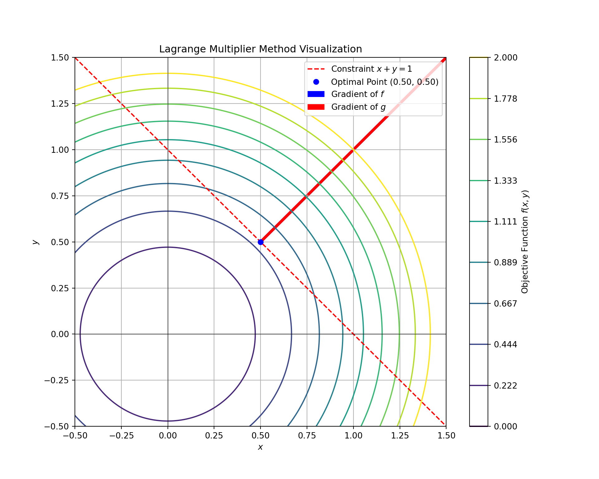

plt.show()

Explanation:

1. Objective Function: The contour plot visualizes \(f(x, y) = x^2 + y^2\) using contour lines, which represent levels of equal function values. The contours help to understand how the objective function behaves over different values of \(x\) and \(y\).

2. Constraint: The dashed red line represents the constraint \(x + y = 1\). This line illustrates the set of points that satisfy the constraint.

3. Optimal Point: The optimal point where the gradients of the objective function and the constraint align is marked with a blue dot. This point is the solution to the constrained optimization problem.

4. Gradients: The blue arrow indicates the gradient of the objective function \(f\) at the optimal point. The red arrow shows the gradient of the constraint \(g\) at the same point. The alignment of these gradients at the optimal point illustrates that the constraint does not change the optimal value of the function. The gradients being parallel is a key feature of the Lagrange Multiplier method, indicating that the solution satisfies the necessary conditions for optimization. (Here, note that the blue gradient line is hide below the red gradient!)

3.9.3.1 Practice Problems

Problem 1:
Maximize \(f(x, y) = x^2 + y^2\)
Subject to \(x + y = 4\)

Solution:
1. Formulate the Lagrangian: \[ \mathcal{L}(x, y, \lambda) = x^2 + y^2 + \lambda (x + y - 4) \]

2. Compute the partial derivatives and set them to zero: \[ \frac{\partial \mathcal{L}}{\partial x} = 2x + \lambda = 0 \quad \Rightarrow \quad \lambda = -2x \] \[ \frac{\partial \mathcal{L}}{\partial y} = 2y + \lambda = 0 \quad \Rightarrow \quad \lambda = -2y \] \[ \frac{\partial \mathcal{L}}{\partial \lambda} = x + y - 4 = 0 \]

3. Equate \(\lambda\) values: \[ -2x = -2y \quad \Rightarrow \quad x = y \]

4. Substitute into constraint: \[ x + x = 4 \quad \Rightarrow \quad 2x = 4 \quad \Rightarrow \quad x = 2 \] \[ y = 2 \]

5. Optimal point: \[ (2, 2) \]

6. Maximum value: \[ f(2, 2) = 2^2 + 2^2 = 8 \]

---

Problem 2:
Minimize \(f(x, y) = x^2 + y^2\)
Subject to \(x + 2y = 6\)

Solution:
1. Formulate the Lagrangian: \[ \mathcal{L}(x, y, \lambda) = x^2 + y^2 + \lambda (x + 2y - 6) \]

2. Compute the partial derivatives and set them to zero: \[ \frac{\partial \mathcal{L}}{\partial x} = 2x + \lambda = 0 \quad \Rightarrow \quad \lambda = -2x \] \[ \frac{\partial \mathcal{L}}{\partial y} = 2y + 2\lambda = 0 \quad \Rightarrow \quad \lambda = -y \] \[ \frac{\partial \mathcal{L}}{\partial \lambda} = x + 2y - 6 = 0 \]

3. Equate \(\lambda\) values: \[ -2x = -y \quad \Rightarrow \quad y = 2x \]

4. Substitute into constraint: \[ x + 2(2x) = 6 \quad \Rightarrow \quad x + 4x = 6 \quad \Rightarrow \quad 5x = 6 \quad \Rightarrow \quad x = \frac{6}{5} \] \[ y = 2 \times \frac{6}{5} = \frac{12}{5} \]

5. Optimal point: \[ \left(\frac{6}{5}, \frac{12}{5}\right) \]

6. Minimum value: \[ f\left(\frac{6}{5}, \frac{12}{5}\right) = \left(\frac{6}{5}\right)^2 + \left(\frac{12}{5}\right)^2 = \frac{36}{25} + \frac{144}{25} = \frac{180}{25} = 7.2 \]

---

Problem 3:
Maximize \(f(x, y) = x + y\)
Subject to \(x^2 + y^2 = 1\)

Solution:
1. Formulate the Lagrangian: \[ \mathcal{L}(x, y, \lambda) = x + y + \lambda (x^2 + y^2 - 1) \]

2. Compute the partial derivatives and set them to zero: \[ \frac{\partial \mathcal{L}}{\partial x} = 1 + 2\lambda x = 0 \quad \Rightarrow \quad \lambda = -\frac{1}{2x} \] \[ \frac{\partial \mathcal{L}}{\partial y} = 1 + 2\lambda y = 0 \quad \Rightarrow \quad \lambda = -\frac{1}{2y} \] \[ \frac{\partial \mathcal{L}}{\partial \lambda} = x^2 + y^2 - 1 = 0 \]

3. Equate \(\lambda\) values: \[ -\frac{1}{2x} = -\frac{1}{2y} \quad \Rightarrow \quad x = y \]

4. Substitute into constraint: \[ x^2 + x^2 = 1 \quad \Rightarrow \quad 2x^2 = 1 \quad \Rightarrow \quad x^2 = \frac{1}{2} \quad \Rightarrow \quad x = \pm \frac{1}{\sqrt{2}} \] \[ y = \pm \frac{1}{\sqrt{2}} \]

5. Optimal points: \[ \left(\frac{1}{\sqrt{2}}, \frac{1}{\sqrt{2}}\right) \text{ and } \left(-\frac{1}{\sqrt{2}}, -\frac{1}{\sqrt{2}}\right) \]

6. Maximum value: \[ f\left(\frac{1}{\sqrt{2}}, \frac{1}{\sqrt{2}}\right) = \frac{1}{\sqrt{2}} + \frac{1}{\sqrt{2}} = \sqrt{2} \] \[ f\left(-\frac{1}{\sqrt{2}}, -\frac{1}{\sqrt{2}}\right) = -\sqrt{2} \]

---

Problem 4:
Minimize \(f(x, y) = x^2 + 2xy + y^2\)
Subject to \(x + y = 2\)

Solution:
1. Formulate the Lagrangian: \[ \mathcal{L}(x, y, \lambda) = x^2 + 2xy + y^2 + \lambda (x + y - 2) \]

2. Compute the partial derivatives and set them to zero: \[ \frac{\partial \mathcal{L}}{\partial x} = 2x + 2y + \lambda = 0 \quad \Rightarrow \quad \lambda = -2x - 2y \] \[ \frac{\partial \mathcal{L}}{\partial y} = 2x + 2y + \lambda = 0 \quad \Rightarrow \quad \lambda = -2x - 2y \] \[ \frac{\partial \mathcal{L}}{\partial \lambda} = x + y - 2 = 0 \]

3. Substitute into constraint: \[ x + y = 2 \]

4. Optimal point: \[ (1, 1) \]

5. Minimum value: \[ f(1, 1) = 1^2 + 2 \times 1 \times 1 + 1^2 = 4 \]

---

Problem 5:
Maximize \(f(x, y) = xy\)
Subject to \(x^2 + y^2 = 1\)

Solution:
1. Formulate the Lagrangian: \[ \mathcal{L}(x, y, \lambda) = xy + \lambda (x^2 + y^2 - 1) \]

2. Compute the partial derivatives and set them to zero: \[ \frac{\partial \mathcal{L}}{\partial x} = y + 2\lambda x = 0 \quad \Rightarrow \quad y = -2\lambda x \] \[ \frac{\partial \mathcal{L}}{\partial y} = x + 2\lambda y = 0 \quad \Rightarrow \quad x = -2\lambda y \] \[ \frac{\partial \mathcal{L}}{\partial \lambda} = x^2 + y^2 - 1 = 0 \]

3. Substitute \(y = -2\lambda x\) into the constraint: \[ x^2 + (-2\lambda x)^2 = 1 \quad \Rightarrow \quad x^2 + 4\lambda^2 x^2 = 1 \quad \Rightarrow \quad x^2(1 + 4\lambda^2) = 1 \] \[ x^2 = \frac{1}{1 + 4\lambda^2} \quad \text{and} \quad y^2 = \frac{4\lambda^2}{1 + 4\lambda^2} \]

4. Optimal points: \[ ( \pm \frac{1}{\sqrt{2}}, \pm \frac{1}{\sqrt{2}} ) \]

5. Maximum value: \[ f\left(\frac{1}{\sqrt{2}}, \frac{1}{\sqrt{2}}\right) = \frac{1}{\sqrt{2}} \times \frac{1}{\sqrt{2}} = \frac{1}{2} \]

---

Problem 6:
Minimize \(f(x, y) = x^2 - 2xy + y^2\)
Subject to \(x + y = 3\)

Solution:
1. Formulate the Lagrangian: \[ \mathcal{L}(x, y, \lambda) = x^2 - 2xy + y^2 + \lambda (x + y - 3) \]

2. Compute the partial derivatives and set them to zero: \[ \frac{\partial \mathcal{L}}{\partial x} = 2x - 2y + \lambda = 0 \quad \Rightarrow \quad \lambda = 2y - 2x \] \[ \frac{\partial \mathcal{L}}{\partial y} = -2x + 2y + \lambda = 0 \quad \Rightarrow \quad \lambda = 2x - 2y \] \[ \frac{\partial \mathcal{L}}{\partial \lambda} = x + y - 3 = 0 \]

3. Substitute into constraint: \[ x + y = 3 \]

4. Optimal point: \[ (1.5, 1.5) \]

5. Minimum value: \[ f(1.5, 1.5) = (1.5)^2 - 2 \times 1.5 \times 1.5 + (1.5)^2 = 0 \]

---

Problem 7:
Maximize \(f(x, y) = x^2 - y^2\)
Subject to \(x^2 + y^2 = 2\)

Solution:
1. Formulate the Lagrangian: \[ \mathcal{L}(x, y, \lambda) = x^2 - y^2 + \lambda (x^2 + y^2 - 2) \]

2. Compute the partial derivatives and set them to zero: \[ \frac{\partial \mathcal{L}}{\partial x} = 2x + 2\lambda x = 0 \quad \Rightarrow \quad x(1 + \lambda) = 0 \] \[ \frac{\partial \mathcal{L}}{\partial y} = -2y + 2\lambda y = 0 \quad \Rightarrow \quad y(1 - \lambda) = 0 \] \[ \frac{\partial \mathcal{L}}{\partial \lambda} = x^2 + y^2 - 2 = 0 \]

3. Case 1: \(x = 0\) \[ y^2 = 2 \quad \Rightarrow \quad y = \pm \sqrt{2} \] \[ f(0, \sqrt{2}) = -2 \] \[ f(0, -\sqrt{2}) = -2 \]

4. Case 2: \(y = 0\) \[ x^2 = 2 \quad \Rightarrow \quad x = \pm \sqrt{2} \] \[ f(\sqrt{2}, 0) = 2 \] \[ f(-\sqrt{2}, 0) = -2 \]

5. Maximum value: \[ 2 \]

---

Problem 8:
Minimize \(f(x, y) = 3x^2 + 4xy + 2y^2\)
Subject to \(x + y = 1\)

Solution:
1. Formulate the Lagrangian: \[ \mathcal{L}(x, y, \lambda) = 3x^2 + 4xy + 2y^2 + \lambda (x + y - 1) \]

2. Compute the partial derivatives and set them to zero: \[ \frac{\partial \mathcal{L}}{\partial x} = 6x + 4y + \lambda = 0 \quad \Rightarrow \quad \lambda = -6x - 4y \] \[ \frac{\partial \mathcal{L}}{\partial y} = 4x + 4y + \lambda = 0 \quad \Rightarrow \quad \lambda = -4x - 4y \] \[ \frac{\partial \mathcal{L}}{\partial \lambda} = x + y - 1 = 0 \]

3. Equate \(\lambda\) values: \[ -6x - 4y = -4x - 4y \quad \Rightarrow \quad -6x = -4x \quad \Rightarrow \quad x = 0 \]

4. Substitute into constraint: \[ x + y = 1 \quad \Rightarrow \quad y = 1 \]

5. Optimal point: \[ (0, 1) \]

6. Minimum value: \[ f(0, 1) = 3(0)^2 + 4(0)(1) + 2(1)^2 = 2 \]

---

Problem 9:
Maximize \(f(x, y) = 2x + 3y\)
Subject to \(x^2 + y^2 = 10\)

Solution:
1. Formulate the Lagrangian: \[ \mathcal{L}(x, y, \lambda) = 2x + 3y + \lambda (x^2 + y^2 - 10) \]

2. Compute the partial derivatives and set them to zero: \[ \frac{\partial \mathcal{L}}{\partial x} = 2 + 2\lambda x = 0 \quad \Rightarrow \quad \lambda = -\frac{1}{x} \] \[ \frac{\partial \mathcal{L}}{\partial y} = 3 + 2\lambda y = 0 \quad \Rightarrow \quad \lambda = -\frac{3}{2y} \] \[ \frac{\partial \mathcal{L}}{\partial \lambda} = x^2 + y^2 - 10 = 0 \]

3. Equate \(\lambda\) values: \[ -\frac{1}{x} = -\frac{3}{2y} \quad \Rightarrow \quad 2y = 3x \quad \Rightarrow \quad y = \frac{3}{2}x \]

4. Substitute into constraint: \[ x^2 + \left(\frac{3}{2}x\right)^2 = 10 \quad \Rightarrow \quad x^2 + \frac{9}{4}x^2 = 10 \quad \Rightarrow \quad \frac{13}{4}x^2 = 10 \quad \Rightarrow \quad x^2 = \frac{40}{13} \] \[ x = \pm \sqrt{\frac{40}{13}} \quad \Rightarrow \quad y = \frac{3}{2} \times \pm \sqrt{\frac{40}{13}} \]

5. Optimal points: \[ \left(\sqrt{\frac{40}{13}}, \frac{3}{2} \sqrt{\frac{40}{13}}\right) \text{ and } \left(-\sqrt{\frac{40}{13}}, -\frac{3}{2} \sqrt{\frac{40}{13}}\right) \]

6. Maximum value: \[ f\left(\sqrt{\frac{40}{13}}, \frac{3}{2} \sqrt{\frac{40}{13}}\right) = 2 \sqrt{\frac{40}{13}} + 3 \times \frac{3}{2} \sqrt{\frac{40}{13}} = \frac{13 \sqrt{40}}{13} = \sqrt{40} \]

---

Problem 10:
Minimize \(f(x, y) = x^3 + y^3\)
Subject to \(x + y = 2\)

Solution:
1. Formulate the Lagrangian: \[ \mathcal{L}(x, y, \lambda) = x^3 + y^3 + \lambda (x + y - 2) \]

2. Compute the partial derivatives and set them to zero: \[ \frac{\partial \mathcal{L}}{\partial x} = 3x^2 + \lambda = 0 \quad \Rightarrow \quad \lambda = -3x^2 \] \[ \frac{\partial \mathcal{L}}{\partial y} = 3y^2 + \lambda = 0 \quad \Rightarrow \quad \lambda = -3y^2 \] \[ \frac{\partial \mathcal{L}}{\partial \lambda} = x + y - 2 = 0 \]

3. Equate \(\lambda\) values: \[ -3x^2 = -3y^2 \quad \Rightarrow \quad x^2 = y^2 \quad \Rightarrow \quad x = \pm y \]

4. Substitute into constraint: \[ x + y = 2 \]

   • Case 1: \(x = y\) \[ 2x = 2 \quad \Rightarrow \quad x = 1 \text{ and } y = 1 \] \[ f(1, 1) = 1^3 + 1^3 = 2 \]

   • Case 2: \(x = -y\) \[ x - x = 2 \text{ (not possible)} \]

5. Optimal point: \[ (1, 1) \]

6. Minimum value: \[ 2 \]

3.9.3.2 Additional Problems

Problem 1: (Minimize the Surface Area of a Box with a Fixed Volume)

A box with a volume of 500 cubic feet needs to be constructed. The goal is to minimize the surface area, where the surface area \(S\) of the box is given by \(S = 2xy + 2xz + 2yz\) and the volume \(V = xyz\).

Solution:

1. Formulate the Lagrangian:

   \[ \mathcal{L}(x, y, z, \lambda) = 2xy + 2xz + 2yz + \lambda (xyz - 500) \]

2. Compute the partial derivatives and set them to zero:

   \[ \frac{\partial \mathcal{L}}{\partial x} = 2y + 2z + \lambda yz = 0 \] \[ \frac{\partial \mathcal{L}}{\partial y} = 2x + 2z + \lambda xz = 0 \] \[ \frac{\partial \mathcal{L}}{\partial z} = 2x + 2y + \lambda xy = 0 \] \[ \frac{\partial \mathcal{L}}{\partial \lambda} = xyz - 500 = 0 \]

3. Solve the system of equations:

   Solving these gives:

   \[ x = y = z = \sqrt[3]{500} \approx 7.937 \]

4. Dimensions:

   \[ x = y = z \approx 7.937 \]

5. Minimum surface area:

   \[ \begin{align*} S &= 2xy + 2xz + 2yz \\ &= 2(7.937 \times 7.937) + 2(7.937 \times 7.937) + 2(7.937 \times 7.937) \\ &= 3 \times 2(7.937 \times 7.937) \\ &= 2 \times 126.6 \\ &= 253.2 \text{ square feet} \end{align*} \]

---

Problem 2: (Minimize the Surface Area of a Prism with a Fixed Volume)

A prism with a volume of 4000 cubic feet has a rectangular base. Find the dimensions of the prism that minimize the surface area.

Solution:

1. Formulate the Lagrangian:

   \[ \mathcal{L}(x, y, h, \lambda) = 2(xy + 2xh + 2yh) + \lambda (xyh - 4000) \]

2. Compute the partial derivatives and set them to zero:

   \[ \frac{\partial \mathcal{L}}{\partial x} = 2y + 2h + \lambda yh = 0 \] \[ \frac{\partial \mathcal{L}}{\partial y} = 2x + 2h + \lambda xh = 0 \] \[ \frac{\partial \mathcal{L}}{\partial h} = 2x + 2y + \lambda xy = 0 \] \[ \frac{\partial \mathcal{L}}{\partial \lambda} = xyh - 4000 = 0 \]

3. Solve the system of equations:

   Solving these gives:

   \[ x = y \approx \sqrt{2000} \approx 44.72, \quad h \approx \frac{4000}{x^2} \approx 2 \]

4. Dimensions:

   \[ x = y \approx 44.72, \quad h \approx 2 \]

5. Minimum surface area:

   \[ \begin{align*} S &= xy + 2xh + 2yh \\ &= 44.72 \times 44.72 + 2(44.72 \times 2) + 2(44.72 \times 2) \\ &= 1990.52 + 179.28 + 179.28 \\ &= 2349.08 \text{ square feet} \end{align*} \]

---

3.9.3.3 (Appendix) Applications in Machine Learning: Ridge, Lasso, and Elastic Net

In the realm of Machine Learning, particularly in linear regression, regularization methods play a crucial role in improving model performance and generalization. Regularization techniques are employed to prevent overfitting, a common issue where a model performs well on training data but poorly on unseen data. The primary goal of regularization is to impose constraints on the model’s complexity, thereby enhancing its ability to generalize.

• Ridge Regression (L2 Regularization): This method adds a penalty proportional to the square of the magnitude of the coefficients. It helps to address multicollinearity and makes the model coefficients more stable by shrinking them towards zero, although it does not necessarily eliminate any coefficients entirely.

• Lasso Regression (L1 Regularization): Unlike Ridge, Lasso regression adds a penalty proportional to the absolute values of the coefficients. This approach not only reduces the magnitude of coefficients but can also drive some coefficients to exactly zero, thus performing automatic feature selection.

• Elastic Net Regression: Combining both L1 and L2 regularization, Elastic Net provides a balanced approach that benefits from the strengths of both Ridge and Lasso. It is particularly useful when there are multiple features correlated with each other.

These regularization methods are implemented using Lagrange multipliers to handle the constraints imposed on the optimization problem. Understanding these techniques is vital for building robust models that are less prone to overfitting and better suited for real-world applications in data analysis and predictive modeling.

3.9.3.4 Ridge, Lasso, and Elastic Net Regularization with Lagrange Multipliers

1. Linear Regression Task Overview

Linear regression aims to model the relationship between a dependent variable \(y\) and one or more independent variables \(X\) by fitting a linear equation to observed data. The goal is to find the coefficients \(\boldsymbol{\beta}\) that minimize the difference between the predicted values and the actual values. The key terms in Linear Regression Model Analysis are:

2. Loss Function: Mean Squared Error

The Mean Squared Error (MSE) is commonly used to measure the performance of a linear regression model:

\[ \text{MSE}(\boldsymbol{\beta}) = \frac{1}{n} \sum_{i=1}^n (y_i - \hat{y}_i)^2 \]

where: - \(y_i\) is the actual value, - \(\hat{y}_i\) is the predicted value, - \(n\) is the number of observations.

3. Possibility of Overfitting

Overfitting occurs when the model is too complex and captures noise in the data rather than the underlying relationship. This often happens with high-dimensional data where the model fits the training data too closely but performs poorly on unseen data.

4. Introduction of Penalty and Its Significance

To address overfitting, regularization techniques add a penalty term to the loss function to constrain the size of the coefficients, making the model simpler and more generalizable. The penalty term discourages large coefficients and helps prevent overfitting.

5. Regularization Methods Using Lagrange Multipliers

Ridge Regression (L2 Regularization)

Penalty: \(\lambda \| \boldsymbol{\beta} \|^2_2\)

Objective Function:

\[ \text{Loss}(\boldsymbol{\beta}) = \text{MSE}(\boldsymbol{\beta}) + \lambda \| \boldsymbol{\beta} \|^2_2 \]

Explanation: Ridge regression adds a penalty proportional to the square of the magnitude of coefficients. This helps manage multicollinearity by shrinking coefficients towards zero but does not set any coefficients exactly to zero.

Lasso Regression (L1 Regularization):

Penalty: \(\lambda \| \boldsymbol{\beta} \|_1\)

Objective Function:

\[ \text{Loss}(\boldsymbol{\beta}) = \text{MSE}(\boldsymbol{\beta}) + \lambda \| \boldsymbol{\beta} \|_1 \]

Explanation: Lasso regression adds a penalty proportional to the absolute value of the coefficients. This promotes sparsity, setting some coefficients exactly to zero, and performs feature selection.

Elastic Net Regression:

Penalty: \(\lambda_1 \| \boldsymbol{\beta} \|_1 + \lambda_2 \| \boldsymbol{\beta} \|^2_2\)

Objective Function:

\[ \text{Loss}(\boldsymbol{\beta}) = \text{MSE}(\boldsymbol{\beta}) + \lambda_1 \| \boldsymbol{\beta} \|_1 + \lambda_2 \| \boldsymbol{\beta} \|^2_2 \]

Explanation: Elastic Net combines both L1 and L2 penalties. This approach balances between Ridge and Lasso, managing multicollinearity and performing feature selection simultaneously.

Here’s how you can visualize Ridge, Lasso, and Elastic Net regression with Python:

import numpy as np
import matplotlib.pyplot as plt
from sklearn.linear_model import Ridge, Lasso, ElasticNet
from sklearn.datasets import make_regression
from sklearn.model_selection import train_test_split

# Generate synthetic data
X, y = make_regression(n_samples=100, n_features=10, noise=0.1, random_state=0)
X_train, X_test, y_train, y_test = train_test_split(X, y, test_size=0.3, random_state=0)

# Define regularization parameters
alpha = 1.0  # Regularization strength for Ridge and Lasso
l1_ratio = 0.5  # Balance between L1 and L2 penalties for Elastic Net

# Create and fit models
ridge = Ridge(alpha=alpha)
lasso = Lasso(alpha=alpha)
elastic_net = ElasticNet(alpha=alpha, l1_ratio=l1_ratio)

ridge.fit(X_train, y_train)

## Ridge()

lasso.fit(X_train, y_train)

## Lasso()

elastic_net.fit(X_train, y_train)

## ElasticNet()

# Predict
y_pred_ridge = ridge.predict(X_test)
y_pred_lasso = lasso.predict(X_test)
y_pred_elastic_net = elastic_net.predict(X_test)

# Plotting
plt.figure(figsize=(15, 10))

## <Figure size 1500x1000 with 0 Axes>

# Ridge Regression
plt.subplot(3, 1, 1)

## <AxesSubplot:>

plt.scatter(y_test, y_pred_ridge, color='blue', label='Ridge')

## <matplotlib.collections.PathCollection object at 0x0000029F5BF75E20>

plt.plot([y_test.min(), y_test.max()], [y_test.min(), y_test.max()], color='red', linestyle='--')

## [<matplotlib.lines.Line2D object at 0x0000029F5BF75D60>]

plt.xlabel('True Values')

## Text(0.5, 0, 'True Values')

plt.ylabel('Predicted Values')

## Text(0, 0.5, 'Predicted Values')

plt.title('Ridge Regression')

## Text(0.5, 1.0, 'Ridge Regression')

plt.legend()

## <matplotlib.legend.Legend object at 0x0000029F5BF83460>

# Lasso Regression
plt.subplot(3, 1, 2)

## <AxesSubplot:>

plt.scatter(y_test, y_pred_lasso, color='green', label='Lasso')

## <matplotlib.collections.PathCollection object at 0x0000029F5BFBEE80>

plt.plot([y_test.min(), y_test.max()], [y_test.min(), y_test.max()], color='red', linestyle='--')

## [<matplotlib.lines.Line2D object at 0x0000029F5BFB5BE0>]

plt.xlabel('True Values')

## Text(0.5, 0, 'True Values')

plt.ylabel('Predicted Values')

## Text(0, 0.5, 'Predicted Values')

plt.title('Lasso Regression')

## Text(0.5, 1.0, 'Lasso Regression')

plt.legend()

## <matplotlib.legend.Legend object at 0x0000029F5BFB5B20>

# Elastic Net Regression
plt.subplot(3, 1, 3)

## <AxesSubplot:>

plt.scatter(y_test, y_pred_elastic_net, color='purple', label='Elastic Net')

## <matplotlib.collections.PathCollection object at 0x0000029F5C004E80>

plt.plot([y_test.min(), y_test.max()], [y_test.min(), y_test.max()], color='red', linestyle='--')

## [<matplotlib.lines.Line2D object at 0x0000029F5BFF9E20>]

plt.xlabel('True Values')

## Text(0.5, 0, 'True Values')

plt.ylabel('Predicted Values')

## Text(0, 0.5, 'Predicted Values')

plt.title('Elastic Net Regression')

## Text(0.5, 1.0, 'Elastic Net Regression')

plt.legend()

## <matplotlib.legend.Legend object at 0x0000029F5BFF9C70>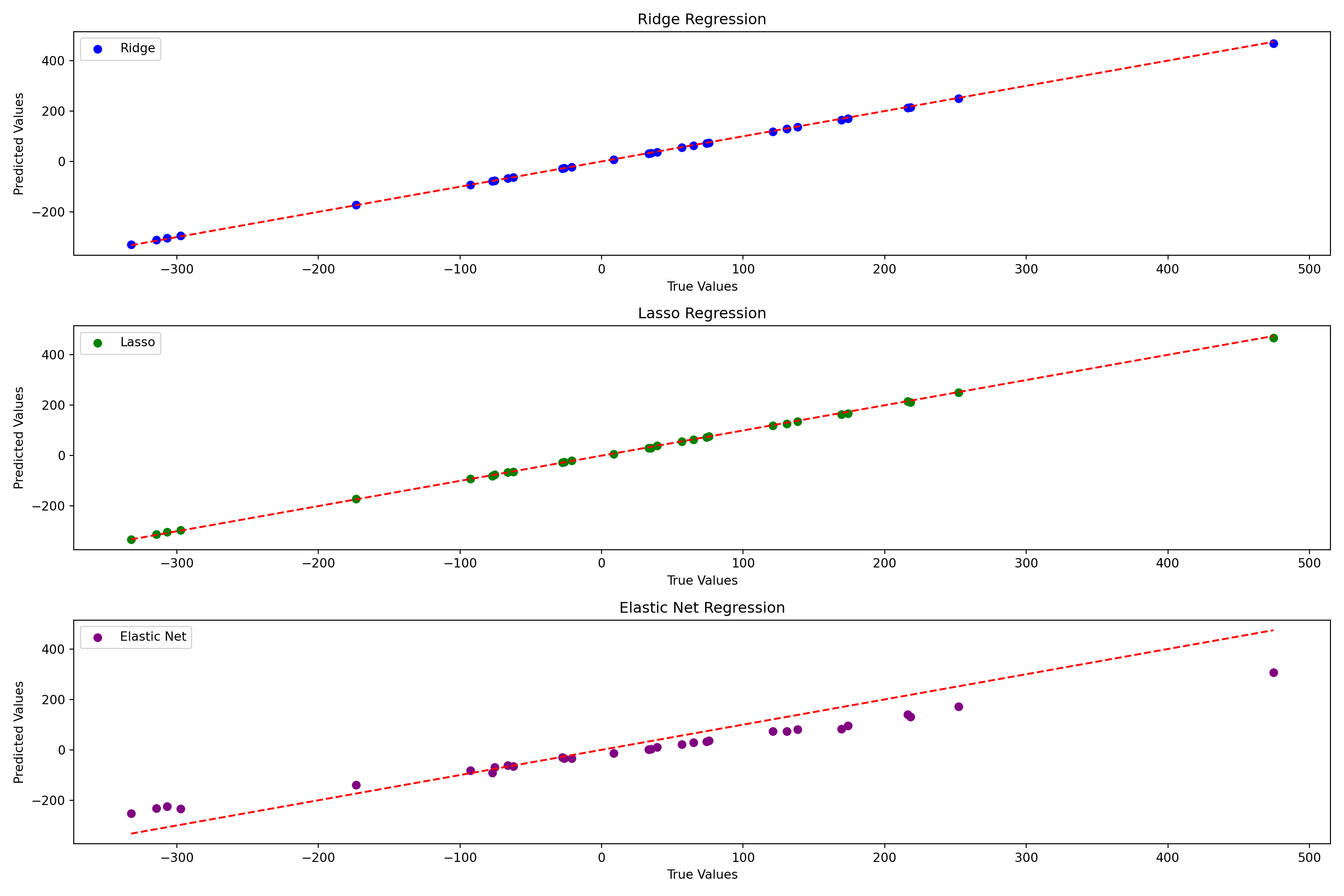

plt.tight_layout()
plt.show()

3.9.4 Method of Steepest Descent

In the Lagrange Multiplier method, we explored how to handle optimization problems subject to constraints. This method effectively finds local extrema of functions when the constraints are linear or can be expressed in a form compatible with Lagrange multipliers. It’s particularly useful when dealing with problems where the objective function is subject to one or more constraints.

However, there are optimization scenarios where the constraints are not explicitly linear or where the problem involves a large number of variables and constraints. In such cases, traditional Lagrange Multiplier methods may become cumbersome or computationally intensive.

This is where the Method of Steepest Descent becomes relevant. Unlike the Lagrange Multiplier method, which incorporates constraints into the optimization process, the Method of Steepest Descent is a more general approach that focuses on minimizing a function iteratively by moving in the direction of the steepest descent (i.e., the negative gradient).

The Method of Steepest Descent, also known as Gradient Descent, is a popular optimization technique used to find the minimum of a function. Here’s a step-by-step explanation of how it works:

1. Initialize the Starting Point: Choose an initial point \(\mathbf{x}_0\) from which the descent will begin. This point can be selected randomly or based on prior knowledge.

2. Compute the Gradient: At each iteration, calculate the gradient \(\nabla f(\mathbf{x}_k)\) of the objective function \(f\) at the current point \(\mathbf{x}_k\). The gradient vector points in the direction of the steepest increase of the function.

3. Determine the Direction of Descent: The direction of steepest descent is the negative gradient, \(-\nabla f(\mathbf{x}_k)\). This direction indicates where the function decreases most rapidly.

4. Update the Current Point: Move from the current point \(\mathbf{x}_k\) to a new point \(\mathbf{x}_{k+1}\) in the direction of the steepest descent. The update is given by: \[ \mathbf{x}_{k+1} = \mathbf{x}_k - \alpha_k \nabla f(\mathbf{x}_k) \] where \(\alpha_k\) is the step size or learning rate.

5. Choose the Step Size: The step size \(\alpha_k\) can be fixed or adjusted dynamically. It controls how far we move in the direction of the gradient. A small step size may result in slow convergence, while a large step size can overshoot the minimum.

6. Check for Convergence: Repeat the above steps until the change in the objective function value or the change in \(\mathbf{x}_k\) is below a predefined threshold, indicating convergence to a minimum.

Application in Minimization of Loss Functions

In the context of Machine Learning, the Method of Steepest Descent is widely used to minimize loss functions. The loss function quantifies the error between the predicted values and the actual values. By applying gradient descent, we iteratively adjust the model parameters to minimize this error, improving the performance and accuracy of the model.

Example: Optimize the function: \[ f(x, y) = x^2 + y^2 \]

Initial Conditions:

• Starting point: \((x_0, y_0) = (2, 2)\)
• Learning rate: \(\alpha = 0.1\)
• Convergence threshold: \(10^{-6}\)
• Maximum iterations: 100

Iteration Table

Iteration	\(x\)	\(y\)	Gradient \(\nabla f(x, y)\)	Updated \(x\)	Updated \(y\)	\(f(x, y)\)
0	2.0000	2.0000	\([4.0000, 4.0000]\)	1.8000	1.8000	6.5000
1	1.8000	1.8000	\([3.6000, 3.6000]\)	1.4400	1.4400	4.1600
2	1.4400	1.4400	\([2.8800, 2.8800]\)	1.1520	1.1520	2.6816
3	1.1520	1.1520	\([2.3040, 2.3040]\)	0.9216	0.9216	1.7170
4	0.9216	0.9216	\([1.8432, 1.8432]\)	0.7373	0.7373	1.0995
5	0.7373	0.7373	\([1.4746, 1.4746]\)	0.5898	0.5898	0.7035
6	0.5898	0.5898	\([1.1796, 1.1796]\)	0.4718	0.4718	0.4503
7	0.4718	0.4718	\([0.9436, 0.9436]\)	0.3774	0.3774	0.2882
8	0.3774	0.3774	\([0.7548, 0.7548]\)	0.3029	0.3029	0.1841
9	0.3029	0.3029	\([0.6058, 0.6058]\)	0.2423	0.2423	0.1178
10	0.2423	0.2423	\([0.4846, 0.4846]\)	0.1938	0.1938	0.0752
11	0.1938	0.1938	\([0.3876, 0.3876]\)	0.1550	0.1550	0.0485
12	0.1550	0.1550	\([0.3100, 0.3100]\)	0.1240	0.1240	0.0310
13	0.1240	0.1240	\([0.2480, 0.2480]\)	0.0992	0.0992	0.0198
14	0.0992	0.0992	\([0.1984, 0.1984]\)	0.0794	0.0794	0.0127
15	0.0794	0.0794	\([0.1588, 0.1588]\)	0.0635	0.0635	0.0081

Note: The iterations continue until the change in the function value or the point is less than the convergence threshold, indicating that the method has effectively converged to the minimum.

Visualization in Python

import numpy as np
import matplotlib.pyplot as plt

# Define the function and its gradient
def f(x, y):
    return x**2 + y**2

def grad_f(x, y):
    return np.array([2*x, 2*y])

# Parameters
alpha = 0.1  # Learning rate
epsilon = 1e-6  # Convergence threshold
max_iterations = 100

# Initialize
x, y = 2, 2  # Starting point
path = [(x, y)]  # To store the path of descent
iteration_data = []  # To store iteration data for table

# Gradient Descent
for i in range(max_iterations):
    gradient = grad_f(x, y)
    x_new, y_new = x - alpha * gradient[0], y - alpha * gradient[1]
    path.append((x_new, y_new))
    
    # Store iteration data
    iteration_data.append([i, x, y, gradient[0], gradient[1], f(x, y)])
    
    # Check for convergence
    if np.linalg.norm([x_new - x, y_new - y]) < epsilon:
        break
    
    x, y = x_new, y_new

# Convert path to numpy array for plotting
path = np.array(path)

# Plotting
X = np.linspace(-3, 3, 100)
Y = np.linspace(-3, 3, 100)
X, Y = np.meshgrid(X, Y)
Z = f(X, Y)

plt.figure(figsize=(10, 6))

## <Figure size 1000x600 with 0 Axes>

contour = plt.contour(X, Y, Z, levels=np.logspace(0, 2, 10), cmap='viridis')
plt.colorbar(contour)

## <matplotlib.colorbar.Colorbar object at 0x0000029F5C10CC40>

plt.plot(path[:, 0], path[:, 1], 'ro-', markersize=5, label='Descent Path')

## [<matplotlib.lines.Line2D object at 0x0000029F5C12C610>]

plt.xlabel('x')

## Text(0.5, 0, 'x')

plt.ylabel('y')

## Text(0, 0.5, 'y')

plt.title('Gradient Descent Optimization')

## Text(0.5, 1.0, 'Gradient Descent Optimization')

plt.legend()

## <matplotlib.legend.Legend object at 0x0000029F5C12CC70>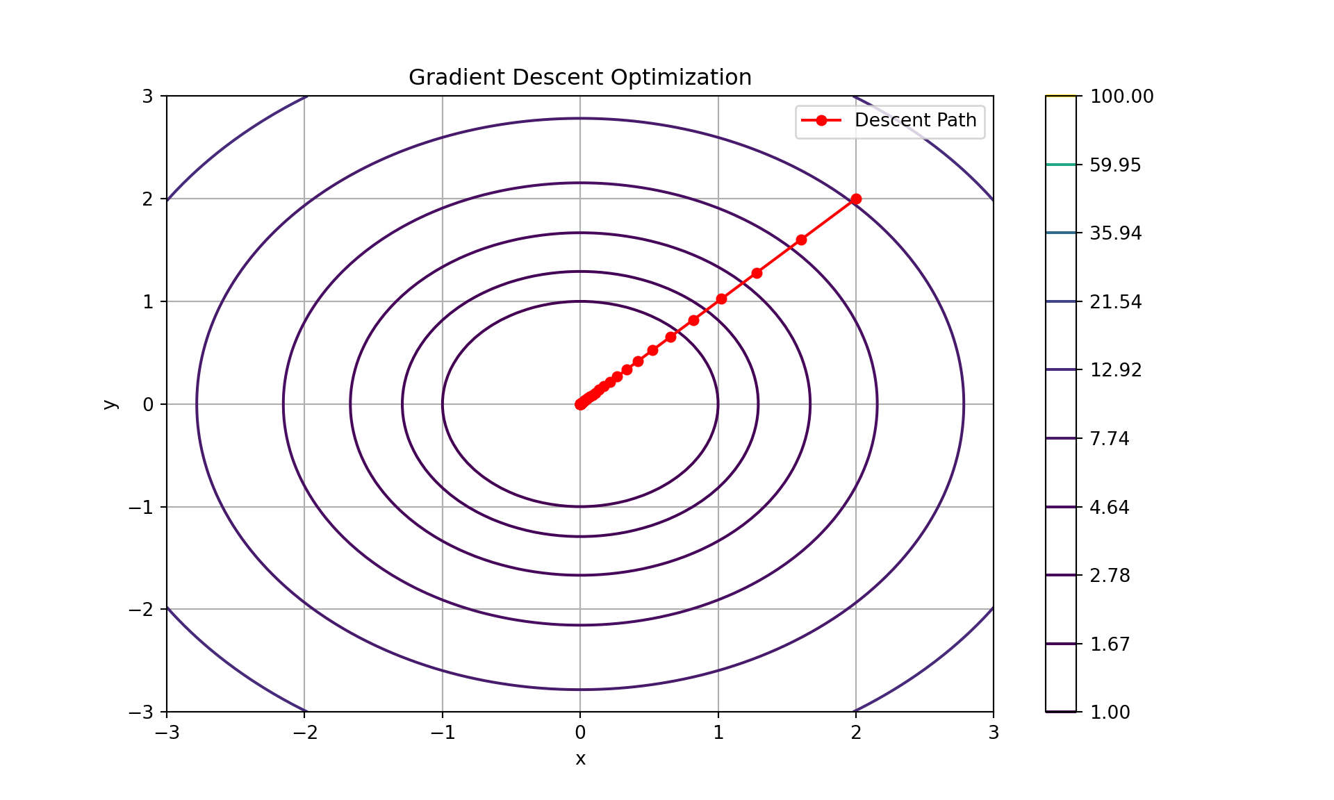

plt.grid(True)
plt.show()

# Print iteration table
print("Iteration Table:")

## Iteration Table:

print(f"{'Iteration':<10}{'x':<10}{'y':<10}{'Gradient x':<15}{'Gradient y':<15}{'f(x, y)'}")

## Iteration x         y         Gradient x     Gradient y     f(x, y)

for data in iteration_data:
    print(f"{data[0]:<10}{data[1]:<10.4f}{data[2]:<10.4f}{data[3]:<15.4f}{data[4]:<15.4f}{data[5]:.4f}")

## 0         2.0000    2.0000    4.0000         4.0000         8.0000
## 1         1.6000    1.6000    3.2000         3.2000         5.1200
## 2         1.2800    1.2800    2.5600         2.5600         3.2768
## 3         1.0240    1.0240    2.0480         2.0480         2.0972
## 4         0.8192    0.8192    1.6384         1.6384         1.3422
## 5         0.6554    0.6554    1.3107         1.3107         0.8590
## 6         0.5243    0.5243    1.0486         1.0486         0.5498
## 7         0.4194    0.4194    0.8389         0.8389         0.3518
## 8         0.3355    0.3355    0.6711         0.6711         0.2252
## 9         0.2684    0.2684    0.5369         0.5369         0.1441
## 10        0.2147    0.2147    0.4295         0.4295         0.0922
## 11        0.1718    0.1718    0.3436         0.3436         0.0590
## 12        0.1374    0.1374    0.2749         0.2749         0.0378
## 13        0.1100    0.1100    0.2199         0.2199         0.0242
## 14        0.0880    0.0880    0.1759         0.1759         0.0155
## 15        0.0704    0.0704    0.1407         0.1407         0.0099
## 16        0.0563    0.0563    0.1126         0.1126         0.0063
## 17        0.0450    0.0450    0.0901         0.0901         0.0041
## 18        0.0360    0.0360    0.0721         0.0721         0.0026
## 19        0.0288    0.0288    0.0576         0.0576         0.0017
## 20        0.0231    0.0231    0.0461         0.0461         0.0011
## 21        0.0184    0.0184    0.0369         0.0369         0.0007
## 22        0.0148    0.0148    0.0295         0.0295         0.0004
## 23        0.0118    0.0118    0.0236         0.0236         0.0003
## 24        0.0094    0.0094    0.0189         0.0189         0.0002
## 25        0.0076    0.0076    0.0151         0.0151         0.0001
## 26        0.0060    0.0060    0.0121         0.0121         0.0001
## 27        0.0048    0.0048    0.0097         0.0097         0.0000
## 28        0.0039    0.0039    0.0077         0.0077         0.0000
## 29        0.0031    0.0031    0.0062         0.0062         0.0000
## 30        0.0025    0.0025    0.0050         0.0050         0.0000
## 31        0.0020    0.0020    0.0040         0.0040         0.0000
## 32        0.0016    0.0016    0.0032         0.0032         0.0000
## 33        0.0013    0.0013    0.0025         0.0025         0.0000
## 34        0.0010    0.0010    0.0020         0.0020         0.0000
## 35        0.0008    0.0008    0.0016         0.0016         0.0000
## 36        0.0006    0.0006    0.0013         0.0013         0.0000
## 37        0.0005    0.0005    0.0010         0.0010         0.0000
## 38        0.0004    0.0004    0.0008         0.0008         0.0000
## 39        0.0003    0.0003    0.0007         0.0007         0.0000
## 40        0.0003    0.0003    0.0005         0.0005         0.0000
## 41        0.0002    0.0002    0.0004         0.0004         0.0000
## 42        0.0002    0.0002    0.0003         0.0003         0.0000
## 43        0.0001    0.0001    0.0003         0.0003         0.0000
## 44        0.0001    0.0001    0.0002         0.0002         0.0000
## 45        0.0001    0.0001    0.0002         0.0002         0.0000
## 46        0.0001    0.0001    0.0001         0.0001         0.0000
## 47        0.0001    0.0001    0.0001         0.0001         0.0000
## 48        0.0000    0.0000    0.0001         0.0001         0.0000
## 49        0.0000    0.0000    0.0001         0.0001         0.0000
## 50        0.0000    0.0000    0.0001         0.0001         0.0000
## 51        0.0000    0.0000    0.0000         0.0000         0.0000
## 52        0.0000    0.0000    0.0000         0.0000         0.0000
## 53        0.0000    0.0000    0.0000         0.0000         0.0000
## 54        0.0000    0.0000    0.0000         0.0000         0.0000
## 55        0.0000    0.0000    0.0000         0.0000         0.0000
## 56        0.0000    0.0000    0.0000         0.0000         0.0000
## 57        0.0000    0.0000    0.0000         0.0000         0.0000
## 58        0.0000    0.0000    0.0000         0.0000         0.0000
## 59        0.0000    0.0000    0.0000         0.0000         0.0000
## 60        0.0000    0.0000    0.0000         0.0000         0.0000

3.9.4.1 Practice Problems

Problem 1: Optimize the function: \[ f(x, y) = x^2 + 2y^2 \]

Initial Conditions: - Starting point: \((x_0, y_0) = (3, 3)\) - Learning rate: \(\alpha = 0.1\) - Convergence threshold: \(10^{-6}\) - Maximum iterations: 50

Iteration Table:

Iteration	x	y	Gradient x	Gradient y	f(x, y)
0	3.0000	3.0000	6.0000	12.0000	15.0000
1	2.4000	1.8000	4.8000	7.2000	8.2800
2	1.9200	1.0800	3.8400	4.3200	4.5180
3	1.5360	0.6480	2.5920	2.5920	2.5456
4	1.2288	0.3888	1.6576	1.5552	1.5394

Solution:

import numpy as np
import matplotlib.pyplot as plt
from mpl_toolkits.mplot3d import Axes3D

# Define the function and its gradient
def f1(x, y):
    return x**2 + 2*y**2

def grad_f1(x, y):
    return np.array([2*x, 4*y])

# Parameters
alpha = 0.1
epsilon = 1e-6
max_iterations = 50

# Initialize
x, y = 3, 3
path = [(x, y)]
iteration_data = []

# Gradient Descent
for i in range(max_iterations):
    gradient = grad_f1(x, y)
    x_new, y_new = x - alpha * gradient[0], y - alpha * gradient[1]
    path.append((x_new, y_new))
    
    # Store iteration data
    if i < 5:  # Only store data for the first 5 iterations
        iteration_data.append([i, x, y, gradient[0], gradient[1], f1(x, y)])
    
    # Check for convergence
    if np.linalg.norm([x_new - x, y_new - y]) < epsilon:
        break
    
    x, y = x_new, y_new

# Convert path to numpy array for plotting
path = np.array(path)

# Plotting 3D
X = np.linspace(-5, 5, 100)
Y = np.linspace(-5, 5, 100)
X, Y = np.meshgrid(X, Y)
Z = f1(X, Y)

fig = plt.figure()
ax = fig.add_subplot(111, projection='3d')
ax.plot_surface(X, Y, Z, cmap='viridis', alpha=0.6)

## <mpl_toolkits.mplot3d.art3d.Poly3DCollection object at 0x0000029F5C1C4640>

ax.plot(path[:, 0], path[:, 1], f1(path[:, 0], path[:, 1]), color='r', marker='o')

## [<mpl_toolkits.mplot3d.art3d.Line3D object at 0x0000029F5C1C4BE0>]

ax.set_xlabel('X axis')

## Text(0.5, 0, 'X axis')

ax.set_ylabel('Y axis')

## Text(0.5, 0.5, 'Y axis')

ax.set_zlabel('f(x, y)')

## Text(0.5, 0, 'f(x, y)')

plt.title('Method of Steepest Descent')

## Text(0.5, 0.92, 'Method of Steepest Descent')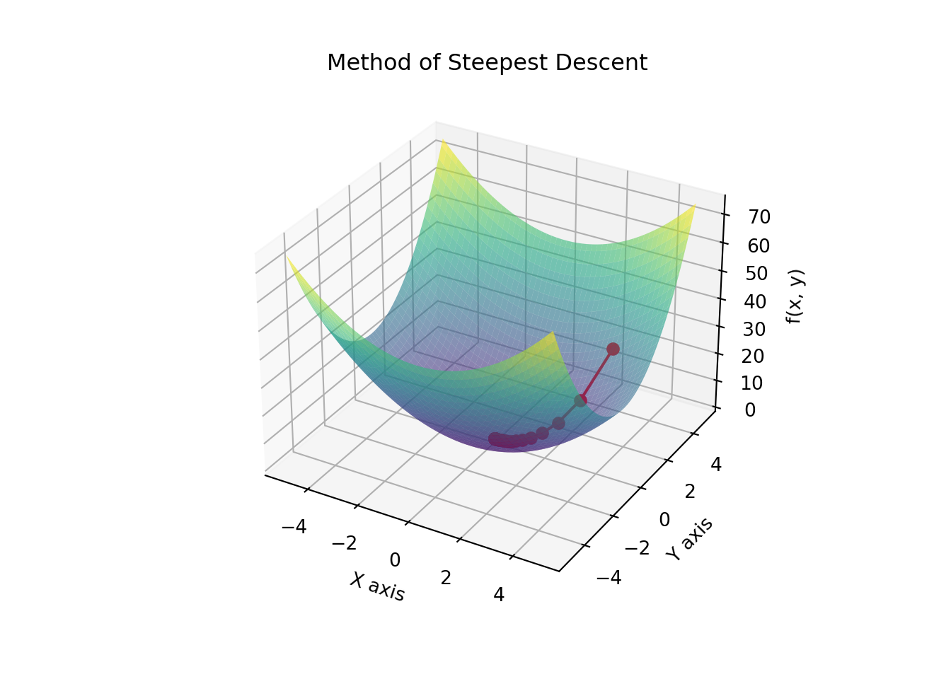

plt.show()

Problem No. 2: Optimize the function:

\[ f(x, y) = 3x^2 + 4y^2 \]

Initial Conditions: - Starting point: \((x_0, y_0) = (4, 2)\) - Learning rate: \(\alpha = 0.05\) - Convergence threshold: \(10^{-6}\) - Maximum iterations: 50

Iteration Table:

Iteration	x	y	Gradient x	Gradient y	f(x, y)
0	4.0000	2.0000	24.0000	16.0000	32.0000
1	2.8000	1.6000	16.8000	12.8000	16.8000
2	1.9600	0.9600	11.7600	7.6800	9.3600
3	1.5680	0.5760	7.1040	4.6080	5.3736
4	1.2544	0.3456	4.5088	2.9440	3.2267

Solution:

import numpy as np
import matplotlib.pyplot as plt
from mpl_toolkits.mplot3d import Axes3D

# Define the function and its gradient
def f2(x, y):
    return 3*x**2 + 4*y**2

def grad_f2(x, y):
    return np.array([6*x, 8*y])

# Parameters
alpha = 0.05
epsilon = 1e-6
max_iterations = 50

# Initialize
x, y = 4, 2
path = [(x, y)]
iteration_data = []

# Gradient Descent
for i in range(max_iterations):
    gradient = grad_f2(x, y)
    x_new, y_new = x - alpha * gradient[0], y - alpha * gradient[1]
    path.append((x_new, y_new))
    
    # Store iteration data
    if i < 5:  # Only store data for the first 5 iterations
        iteration_data.append([i, x, y, gradient[0], gradient[1], f2(x, y)])
    
    # Check for convergence
    if np.linalg.norm([x_new - x, y_new - y]) < epsilon:
        break
    
    x, y = x_new, y_new

# Convert path to numpy array for plotting
path = np.array(path)

# Plotting 3D
X = np.linspace(-5, 5, 100)
Y = np.linspace(-5, 5, 100)
X, Y = np.meshgrid(X, Y)
Z = f2(X, Y)

fig = plt.figure()
ax = fig.add_subplot(111, projection='3d')
ax.plot_surface(X, Y, Z, cmap='plasma', alpha=0.6)

## <mpl_toolkits.mplot3d.art3d.Poly3DCollection object at 0x0000029F59DF9820>

ax.plot(path[:, 0], path[:, 1], f2(path[:, 0], path[:, 1]), color='r', marker='o')

## [<mpl_toolkits.mplot3d.art3d.Line3D object at 0x0000029F59DF93D0>]

ax.set_xlabel('X axis')

## Text(0.5, 0, 'X axis')

ax.set_ylabel('Y axis')

## Text(0.5, 0.5, 'Y axis')

ax.set_zlabel('f(x, y)')

## Text(0.5, 0, 'f(x, y)')

plt.title('Method of Steepest Descent')

## Text(0.5, 0.92, 'Method of Steepest Descent')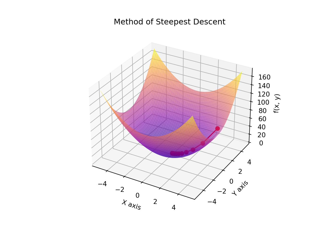

plt.show()

Problem No. 3: Optimize the function:

\[ f(x, y) = x^2 + xy + y^2 \]

Initial Conditions: - Starting point: \((x_0, y_0) = (3, 1)\) - Learning rate: \(\alpha = 0.1\) - Convergence threshold: \(10^{-6}\) - Maximum iterations: 50

Iteration Table:

Iteration	x	y	Gradient x	Gradient y	f(x, y)
0	3.0000	1.0000	7.0000	4.0000	13.0000
1	2.3000	0.6000	4.6000	2.2000	6.5600
2	1.6600	0.3800	2.9200	1.6400	3.5200
3	1.2800	0.2360	1.8880	1.1760	1.9200
4	0.9920	0.1480	1.2100	0.7840	1.1050

Solution:

import numpy as np
import matplotlib.pyplot as plt
from mpl_toolkits.mplot3d import Axes3D

# Define the function and its gradient
def f3(x, y):
    return x**2 + x*y + y**2

def grad_f3(x, y):
    return np.array([2*x + y, x + 2*y])

# Parameters
alpha = 0.1
epsilon = 1e-6
max_iterations = 50

# Initialize
x, y = 3, 1
path = [(x, y)]
iteration_data = []

# Gradient Descent
for i in range(max_iterations):
    gradient = grad_f3(x, y)
    x_new, y_new = x - alpha * gradient[0], y - alpha * gradient[1]
    path.append((x_new, y_new))
    
    # Store iteration data
    if i < 5:  # Only store data for the first 5 iterations
        iteration_data.append([i, x, y, gradient[0], gradient[1], f3(x, y)])
    
    # Check for convergence
    if np.linalg.norm([x_new - x, y_new - y]) < epsilon:
        break
    
    x, y = x_new, y_new

# Convert path to numpy array for plotting
path = np.array(path)

# Plotting 3D
X = np.linspace(-5, 5, 100)
Y = np.linspace(-5, 5, 100)
X, Y = np.meshgrid(X, Y)
Z = f3(X, Y)

fig = plt.figure()
ax = fig.add_subplot(111, projection='3d')
ax.plot_surface(X, Y, Z, cmap='plasma', alpha=0.6)

## <mpl_toolkits.mplot3d.art3d.Poly3DCollection object at 0x0000029F5C230640>

ax.plot(path[:, 0], path[:, 1], f3(path[:, 0], path[:, 1]), color='r', marker='o')

## [<mpl_toolkits.mplot3d.art3d.Line3D object at 0x0000029F5C22BF10>]

ax.set_xlabel('X axis')

## Text(0.5, 0, 'X axis')

ax.set_ylabel('Y axis')

## Text(0.5, 0.5, 'Y axis')

ax.set_zlabel('f(x, y)')

## Text(0.5, 0, 'f(x, y)')

plt.title('Method of Steepest Descent')

## Text(0.5, 0.92, 'Method of Steepest Descent')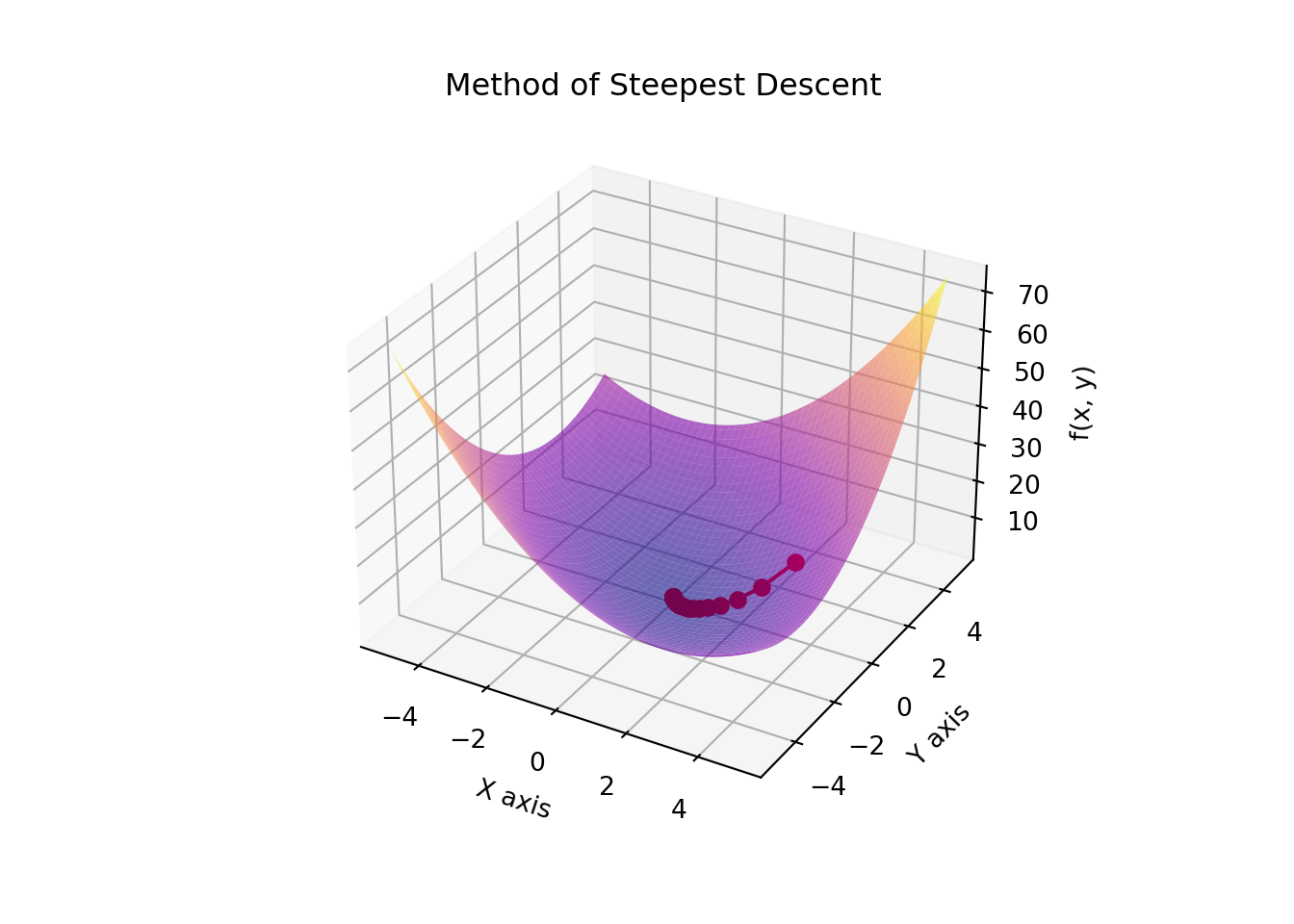

plt.show()

Problem No. 4: Optimize the function:

\[ f(x, y) = 2x^2 + 3xy + 4y^2 \]

Initial Conditions: - Starting point: \((x_0, y_0) = (-2, 2)\) - Learning rate: \(\alpha = 0.05\) - Convergence threshold: \(10^{-6}\) - Maximum iterations: 50

Iteration Table:

Iteration	x	y	Gradient x	Gradient y	f(x, y)
0	-2.0000	2.0000	-16.0000	4.0000	16.0000
1	-0.8000	1.8000	-9.0000	2.8000	7.1200
2	-0.1100	1.5560	-4.2320	1.5720	2.5120
3	0.0390	1.3530	-1.8700	0.9630	0.8160
4	0.1130	1.1520	-0.8990	0.6220	0.3300

Solution:

import numpy as np
import matplotlib.pyplot as plt
from mpl_toolkits.mplot3d import Axes3D

# Define the function and its gradient
def f4(x, y):
    return 2*x**2 + 3*x*y + 4*y**2

def grad_f4(x, y):
    return np.array([4*x + 3*y, 3*x + 8*y])

# Parameters
alpha = 0.05
epsilon = 1e-6
max_iterations = 50

# Initialize
x, y = -2, 2
path = [(x, y)]
iteration_data = []

# Gradient Descent
for i in range(max_iterations):
    gradient = grad_f4(x, y)
    x_new, y_new = x - alpha * gradient[0], y - alpha * gradient[1]
    path.append((x_new, y_new))
    
    # Store iteration data
    if i < 5:  # Only store data for the first 5 iterations
        iteration_data.append([i, x, y, gradient[0], gradient[1], f4(x, y)])
    
    # Check for convergence
    if np.linalg.norm([x_new - x, y_new - y]) < epsilon:
        break
    
    x, y = x_new, y_new

# Convert path to numpy array for plotting
path = np.array(path)

# Plotting 3D
X = np.linspace(-5, 5, 100)
Y = np.linspace(-5, 5, 100)
X, Y = np.meshgrid(X, Y)
Z = f4(X, Y)

fig = plt.figure()
ax = fig.add_subplot(111, projection='3d')
ax.plot_surface(X, Y, Z, cmap='viridis', alpha=0.6)

## <mpl_toolkits.mplot3d.art3d.Poly3DCollection object at 0x0000029F5B5C7340>

ax.plot(path[:, 0], path[:, 1], f4(path[:, 0], path[:, 1]), color='r', marker='o')

## [<mpl_toolkits.mplot3d.art3d.Line3D object at 0x0000029F5B5C76A0>]

ax.set_xlabel('X axis')

## Text(0.5, 0, 'X axis')

ax.set_ylabel('Y axis')

## Text(0.5, 0.5, 'Y axis')

ax.set_zlabel('f(x, y)')

## Text(0.5, 0, 'f(x, y)')

plt.title('Method of Steepest Descent')

## Text(0.5, 0.92, 'Method of Steepest Descent')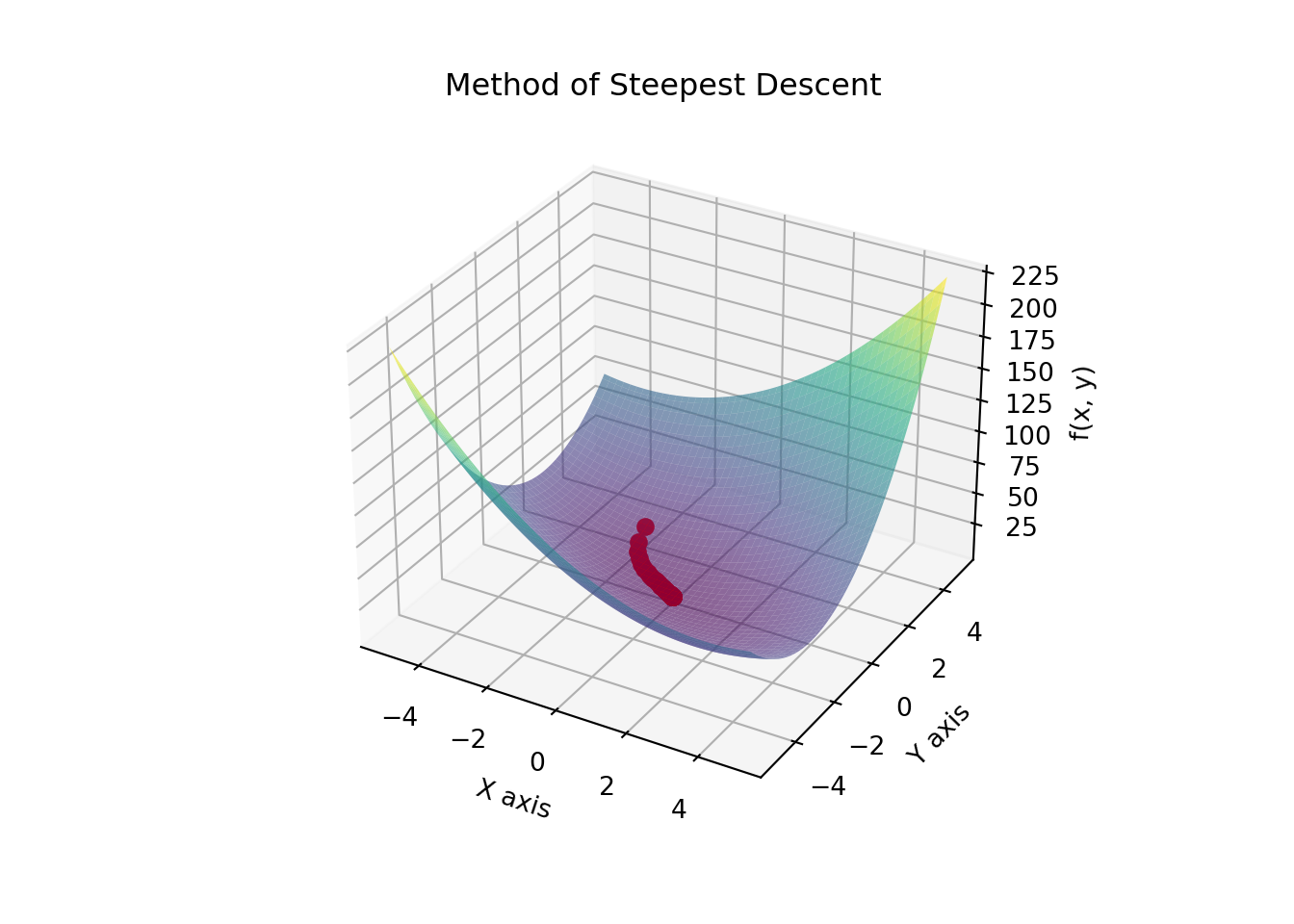

plt.show()

Problem No. 5: Optimize the function:

\[ f(x, y) = x^2 + 2xy + y^2 - 4x - 6y + 10 \]

Initial Conditions: - Starting point: \((x_0, y_0) = (1, 1)\) - Learning rate: \(\alpha = 0.1\) - Convergence threshold: \(10^{-6}\) - Maximum iterations: 50

Iteration Table:

Iteration	x	y	Gradient x	Gradient y	f(x, y)
0	1.0000	1.0000	-2.0000	-4.0000	4.0000
1	2.2000	2.4000	-0.8000	-1.6000	1.2800
2	2.6800	2.8400	-0.3360	-0.6720	0.4550
3	2.8224	2.9520	-0.1488	-0.2976	0.1488
4	2.8910	2.9932	-0.0650	-0.1298	0.0494

Solution:

import numpy as np
import matplotlib.pyplot as plt
from mpl_toolkits.mplot3d import Axes3D

# Define the function and its gradient
def f5(x, y):
    return x**2 + 2*x*y + y**2 - 4*x - 6*y + 10

def grad_f5(x, y):
    return np.array([2*x + 2*y - 4, 2*x + 2*y - 6])

# Parameters
alpha = 0.1
epsilon = 1e-6
max_iterations = 50

# Initialize
x, y = 1, 1
path = [(x, y)]
iteration_data = []

# Gradient Descent
for i in range(max_iterations):
    gradient = grad_f5(x, y)
    x_new, y_new = x - alpha * gradient[0], y - alpha * gradient[1]
    path.append((x_new, y_new))
    
    # Store iteration data
    if i < 5:  # Only store data for the first 5 iterations
        iteration_data.append([i, x, y, gradient[0], gradient[1], f5(x, y)])
    
    # Check for convergence
    if np.linalg.norm([x_new - x, y_new - y]) < epsilon:
        break
    
    x, y = x_new, y_new

# Convert path to numpy array for plotting
path = np.array(path)

# Plotting 3D
X = np.linspace(-1, 4, 100)
Y = np.linspace(-1, 4, 100)
X, Y = np.meshgrid(X, Y)
Z = f5(X, Y)

fig = plt.figure()
ax = fig.add_subplot(111, projection='3d')
ax.plot_surface(X, Y, Z, cmap='plasma', alpha=0.6)

## <mpl_toolkits.mplot3d.art3d.Poly3DCollection object at 0x0000029F5E42E7C0>

ax.plot(path[:, 0], path[:, 1], f5(path[:, 0], path[:, 1]), color='r', marker='o')

## [<mpl_toolkits.mplot3d.art3d.Line3D object at 0x0000029F5E42E7F0>]

ax.set_xlabel('X axis')

## Text(0.5, 0, 'X axis')

ax.set_ylabel('Y axis')

## Text(0.5, 0.5, 'Y axis')

ax.set_zlabel('f(x, y)')

## Text(0.5, 0, 'f(x, y)')

plt.title('Method of Steepest Descent')

## Text(0.5, 0.92, 'Method of Steepest Descent')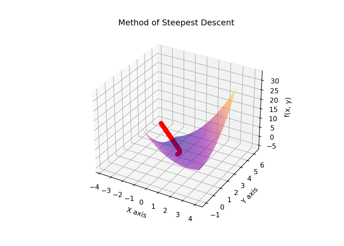

plt.show()

### Linear Programming Problem (LPP)

In this section, we are going to discuss a special algorithm designed to solve linear optimization problems with linear constraints. Linear Programming (LP) is a mathematical method used to optimize a linear objective function subject to linear equality and inequality constraints. This approach is highly valuable in various fields for making optimal decisions within constrained environments.

Historical Context

The formal development of linear programming began with George Dantzig’s work in the 1940s. Dantzig, a mathematician and operations researcher, introduced the simplex method, which was a significant breakthrough in solving optimization problems. Initially applied to military logistics during World War II, this method efficiently addressed complex resource allocation issues.

The simplex method, developed by Dantzig, paved the way for future advancements in optimization. In the 1980s, Narendra Karmarkar introduced interior-point methods, offering an alternative to the simplex method for solving large-scale LP problems. These advancements have cemented linear programming as a critical tool in operations research, economics, engineering, and other fields.

Applications of Linear Programming

Linear Programming has extensive applications in various domains:

• Operations Research: LP is used to optimize logistics and supply chain management, including transportation routes, inventory levels, and resource allocation. For example, a company might use LP to minimize transportation costs while meeting delivery deadlines and capacity constraints.

• Economics: In resource allocation problems, LP helps to maximize profit or minimize cost. It is used in production planning, cost minimization, and other economic decisions where resources are limited.

• Engineering: LP aids in designing efficient manufacturing processes and optimizing production schedules. Engineers use LP to solve problems related to workforce scheduling, equipment usage, and materials management.

• Finance: In finance, LP is used for portfolio optimization to manage investment risk and return. Investors allocate funds across assets to achieve the best possible return for a given level of risk.

• Transportation: LP is used in network optimization for designing efficient routing systems for public transportation, freight delivery, and urban planning. It helps minimize travel time and operational costs while adhering to constraints.

Differences from Previously Discussed Methods

3.9.4.2 Lagrange Multipliers vs. Linear Programming

• Scope of Application: Lagrange Multipliers are used for constrained optimization problems with differentiable objective functions and constraints. They help find local extrema subject to equality constraints. Linear Programming, in contrast, is applied to problems with linear relationships and constraints, covering a broader range of optimization issues that may not be differentiable.

• Mathematical Approach: Lagrange Multipliers transform a constrained problem into an unconstrained one by incorporating constraints into the objective function using additional variables. Linear Programming involves linear constraints and objectives, using methods like the simplex algorithm to explore feasible regions and find the optimal solution.

Method of Steepest Descent vs. Linear Programming - Optimization Type: The Method of Steepest Descent is used for unconstrained optimization problems, focusing on minimizing a function by moving in the direction of the negative gradient. Linear Programming deals with linear constraints and objectives, using geometric methods to find the optimal solution.

• Algorithmic Differences: The Method of Steepest Descent iteratively refines an initial guess based on gradient information. Linear Programming uses algorithms like the simplex method or interior-point methods to systematically explore feasible solutions and determine the optimal point.

3.9.4.3 Formulation of a Linear Programming Problem (LPP)

To illustrate the formulation of a Linear Programming Problem (LPP), consider the following context:

Context: Resource Allocation in Manufacturing: Imagine a company that manufactures two types of products: Product A and Product B. The company has limited resources and wants to determine the optimal number of each product to produce in order to maximize its profit. Each product requires different amounts of resources and generates different profits.

Problem Statement

The company wants to maximize its total profit subject to constraints on the available resources. Let’s denote:

• \(x_1\) = Number of units of Product A produced
• \(x_2\) = Number of units of Product B produced

The objective is to maximize the total profit, which is given by:

\[ \text{Profit} = c_1 x_1 + c_2 x_2 \]

where \(c_1\) and \(c_2\) are the profits per unit of Product A and Product B, respectively.

Constraints

The company has constraints on the resources available. Suppose:

1. Resource 1 Constraint: Each unit of Product A requires \(a_1\) units of Resource 1, and each unit of Product B requires \(a_2\) units of Resource 1. The total available units of Resource 1 are \(b_1\). Therefore, the constraint is:

   \[ a_1 x_1 + a_2 x_2 \leq b_1 \]

2. Resource 2 Constraint: Each unit of Product A requires \(b_1\) units of Resource 2, and each unit of Product B requires \(b_2\) units of Resource 2. The total available units of Resource 2 are \(b_2\). Therefore, the constraint is:

   \[ b_1 x_1 + b_2 x_2 \leq b_2 \]

3. Non-negativity Constraints: The company cannot produce a negative number of products, so:

   \[ x_1 \geq 0 \] \[ x_2 \geq 0 \]

Formulation of the LPP

Putting it all together, the Linear Programming Problem can be formulated as follows:

Objective Function:

\[ \text{Maximize } Z = c_1 x_1 + c_2 x_2 \]

Subject to:

\[\begin{align*} a_1 x_1 + a_2 x_2 &\leq b_1\\ b_1 x_1 + b_2 x_2 &\leq b_2\\ x_1 &\geq 0\\ x_2 &\geq 0 \end{align*}\]

Where:

• \(c_1\) and \(c_2\) are the profit coefficients for Product A and Product B, respectively.
• \(a_1\), \(a_2\), \(b_1\), and \(b_2\) are the resource requirements and availability.
• \(x_1\) and \(x_2\) are the decision variables representing the number of units to produce.

Example 1: A furniture company manufactures tables and chairs. Each table yields a profit of $50 and requires 4 hours of labor and 3 units of material. Each chair provides a profit of $30 and needs 2 hours of labor and 2 units of material. The company has a maximum of 160 labor hours and 120 units of material available. The objective is to determine the optimal number of tables and chairs to produce in order to maximize profit while adhering to these resource constraints. Formulate a mathematical model to this problem.

Mathematical Formulation:

1. Define the Decision Variables:

   Let \(x_1\) be the number of tables produced.
   Let \(x_2\) be the number of chairs produced.

2. Objective Function:

   The goal is to maximize the total profit \(Z\):

   \[ \text{Maximize } Z = 50x_1 + 30x_2 \]

3. Constraints:

   • Labor Constraint: Each table requires 4 hours and each chair requires 2 hours. The total labor hours available are 160 hours:

     \[ 4x_1 + 2x_2 \leq 160 \]

   • Material Constraint: Each table requires 3 units of material and each chair requires 2 units of material. The total material units available are 120 units:

     \[ 3x_1 + 2x_2 \leq 120 \]

   • Non-negativity Constraints: The number of tables and chairs cannot be negative:

     \[ x_1 \geq 0 \] \[ x_2 \geq 0 \]

*Complete model:**

\[ \text{Maximize } Z = 50x_1 + 30x_2 \]

Subject to: \[\begin{align*} 4x_1 + 2x_2 &\leq 160\\ 3x_1 + 2x_2 &\leq 120\\ x_1,x_2&\geq 0 \end{align*}\]

3.9.5 Practice Problems:

Problem 1:

A bakery produces two types of bread, Type A and Type B. Each loaf of Type A requires 2 hours of baking and 3 units of flour. Each loaf of Type B requires 1 hour of baking and 2 units of flour. The bakery has 80 hours of baking time and 60 units of flour available. Type A sells for $4 and Type B sells for $3. Formulate the linear programming problem to maximize profit.

Solution:

Define the decision variables: - Let \(x_1\) be the number of loaves of Type A produced. - Let \(x_2\) be the number of loaves of Type B produced.

Objective function: \[ \text{Maximize } Z = 4x_1 + 3x_2 \]

Subject to: \[\begin{align*} 2x_1 + x_2 &\leq 80 \\ 3x_1 + 2x_2 &\leq 60 \\ x_1, x_2 &\geq 0 \end{align*}\]

Problem 2:

A factory produces two products, Product X and Product Y. Each unit of Product X requires 5 hours of machine time and 2 units of raw material. Each unit of Product Y requires 3 hours of machine time and 4 units of raw material. The factory has 120 hours of machine time and 100 units of raw material available. Product X yields $10 profit and Product Y yields $15 profit. Formulate the linear programming problem to maximize profit.

Solution:

Define the decision variables: - Let \(x_1\) be the number of units of Product X. - Let \(x_2\) be the number of units of Product Y.

Objective function: \[ \text{Maximize } Z = 10x_1 + 15x_2 \]

Subject to: \[\begin{align*} 5x_1 + 3x_2 &\leq 120 \\ 2x_1 + 4x_2 &\leq 100 \\ x_1, x_2 &\geq 0 \end{align*}\]

Problem 3:

A company produces two types of widgets, Widget A and Widget B. Each Widget A requires 3 hours of production time and 2 units of raw materials. Each Widget B requires 4 hours of production time and 3 units of raw materials. The company has 150 hours of production time and 200 units of raw materials. Widget A sells for $5 and Widget B sells for $6. Formulate the linear programming problem to maximize revenue.

Solution:

Define the decision variables: - Let \(x_1\) be the number of Widget A produced. - Let \(x_2\) be the number of Widget B produced.

Objective function: \[ \text{Maximize } Z = 5x_1 + 6x_2 \]

Subject to: \[\begin{align*} 3x_1 + 4x_2 &\leq 150 \\ 2x_1 + 3x_2 &\leq 200 \\ x_1, x_2 &\geq 0 \end{align*}\]

Problem 4:

A manufacturer makes two types of gadgets, Gadget A and Gadget B. Each Gadget A requires 6 hours of assembly and 4 units of parts. Each Gadget B requires 5 hours of assembly and 3 units of parts. The manufacturer has 180 hours of assembly time and 150 units of parts. Gadget A brings in $8 profit and Gadget B brings in $7 profit. Formulate the linear programming problem to maximize profit.

Solution:

Define the decision variables: - Let \(x_1\) be the number of Gadget A produced. - Let \(x_2\) be the number of Gadget B produced.

Objective function: \[ \text{Maximize } Z = 8x_1 + 7x_2 \]

Subject to: \[\begin{align*} 6x_1 + 5x_2 &\leq 180 \\ 4x_1 + 3x_2 &\leq 150 \\ x_1, x_2 &\geq 0 \end{align*}\]

Problem 5:

A restaurant offers two types of meals, Meal A and Meal B. Meal A requires 2 hours of kitchen time and 1 unit of ingredients. Meal B requires 1 hour of kitchen time and 2 units of ingredients. The restaurant has 60 hours of kitchen time and 40 units of ingredients available. Meal A sells for $12 and Meal B sells for $10. Formulate the linear programming problem to maximize profit.

Solution:

Define the decision variables: - Let \(x_1\) be the number of Meal A prepared. - Let \(x_2\) be the number of Meal B prepared.

Objective function: \[ \text{Maximize } Z = 12x_1 + 10x_2 \]

Subject to: \[\begin{align*} 2x_1 + x_2 &\leq 60 \\ x_1 + 2x_2 &\leq 40 \\ x_1, x_2 &\geq 0 \end{align*}\]

Problem 6:

A company produces two products, Product A and Product B. Each unit of Product A requires 7 hours of labor and 5 units of raw material. Each unit of Product B requires 4 hours of labor and 6 units of raw material. The company has 200 hours of labor and 180 units of raw material available. Product A provides $20 profit and Product B provides $15 profit. Formulate the linear programming problem to maximize profit.

Solution:

Define the decision variables: - Let \(x_1\) be the number of units of Product A. - Let \(x_2\) be the number of units of Product B.

Objective function: \[ \text{Maximize } Z = 20x_1 + 15x_2 \]

Subject to: \[\begin{align*} 7x_1 + 4x_2 &\leq 200 \\ 5x_1 + 6x_2 &\leq 180 \\ x_1, x_2 &\geq 0 \end{align*}\]

Problem 7:

A firm manufactures two types of electronic devices, Device X and Device Y. Each Device X requires 5 hours of machine time and 4 units of materials. Each Device Y requires 3 hours of machine time and 6 units of materials. The firm has 100 hours of machine time and 120 units of materials available. Device X yields $30 profit and Device Y yields $25 profit. Formulate the linear programming problem to maximize profit.

Solution:

Define the decision variables: - Let \(x_1\) be the number of Device X produced. - Let \(x_2\) be the number of Device Y produced.

Objective function: \[ \text{Maximize } Z = 30x_1 + 25x_2 \]

Subject to: \[\begin{align*} 5x_1 + 3x_2 &\leq 100 \\ 4x_1 + 6x_2 &\leq 120 \\ x_1, x_2 &\geq 0 \end{align*}\]

Problem 8:

A factory produces two types of toys, Toy A and Toy B. Each Toy A requires 4 hours of labor and 5 units of materials. Each Toy B requires 6 hours of labor and 3 units of materials. The factory has 150 hours of labor and 120 units of materials available. Toy A provides $18 profit and Toy B provides $22 profit. Formulate the linear programming problem to maximize profit.

Solution:

Define the decision variables: - Let \(x_1\) be the number of Toy A produced. - Let \(x_2\) be the number of Toy B produced.

Objective function: \[ \text{Maximize } Z = 18x_1 + 22x_2 \]

Subject to: \[\begin{align*} 4x_1 + 6x_2 &\leq 150 \\ 5x_1 + 3x_2 &\leq 120 \\ x_1, x_2 &\geq 0 \end{align*}\]

Problem 9:

A plant produces two types of chemicals, Chemical A and Chemical B. Each unit of Chemical A requires 8 hours of processing and 5 units of raw materials. Each unit of Chemical B requires 6 hours of processing and 7 units of raw materials. The plant has 200 hours of processing time and 150 units of raw materials available. Chemical A yields $40 profit and Chemical B yields $50 profit. Formulate the linear programming problem to maximize profit.

Solution:

Define the decision variables: - Let \(x_1\) be the number of units of Chemical A. - Let \(x_2\) be the number of units of Chemical B.

Objective function: \[ \text{Maximize } Z = 40x_1 + 50x_2 \]

Subject to: \[\begin{align*} 8x_1 + 6x_2 &\leq 200 \\ 5x_1 + 7x_2 &\leq 150 \\ x_1, x_2 &\geq 0 \end{align*}\]

Problem 10:

A construction company builds two types of structures, Structure A and Structure B. Each Structure A requires 3 hours of labor and 4 units of materials. Each Structure B requires 5 hours of labor and 2 units of materials. The company has 120 hours of labor and 80 units of materials available. Structure A generates $25 profit and Structure B generates $30 profit. Formulate the linear programming problem to maximize profit.

Solution:

Define the decision variables: - Let \(x_1\) be the number of Structure A built. - Let \(x_2\) be the number of Structure B built.

Objective function: \[ \text{Maximize } Z = 25x_1 + 30x_2 \]

Subject to: \[\begin{align*} 3x_1 + 5x_2 &\leq 120 \\ 4x_1 + 2x_2 &\leq 80 \\ x_1, x_2 &\geq 0 \end{align*}\] Problem 11:

A software development company is working on two projects, Project X and Project Y. Each Project X requires 10 hours of developer time and 8 hours of testing. Each Project Y requires 6 hours of developer time and 12 hours of testing. The company has 400 hours of developer time and 360 hours of testing available. Project X generates $50,000 in revenue and Project Y generates $40,000 in revenue. Formulate the linear programming problem to maximize revenue.

Solution:

Define the decision variables: - Let \(x_1\) be the number of Project X completed. - Let \(x_2\) be the number of Project Y completed.

Objective function: \[ \text{Maximize } Z = 50000x_1 + 40000x_2 \]

Subject to: \[\begin{align*} 10x_1 + 6x_2 &\leq 400 \\ 8x_1 + 12x_2 &\leq 360 \\ x_1, x_2 &\geq 0 \end{align*}\]

Problem 12:

A data center is running two types of tasks, Task A and Task B. Each Task A requires 3 hours of CPU time and 2 hours of memory usage. Each Task B requires 4 hours of CPU time and 5 hours of memory usage. The data center has 120 hours of CPU time and 100 hours of memory usage available. Task A brings $200 in profit and Task B brings $300 in profit. Formulate the linear programming problem to maximize profit.

Solution:

Define the decision variables: - Let \(x_1\) be the number of Task A executed. - Let \(x_2\) be the number of Task B executed.

Objective function: \[ \text{Maximize } Z = 200x_1 + 300x_2 \]

Subject to: \[\begin{align*} 3x_1 + 4x_2 &\leq 120 \\ 2x_1 + 5x_2 &\leq 100 \\ x_1, x_2 &\geq 0 \end{align*}\]

3.9.6 Simplex Method

The Simplex method is an algorithm used for solving linear programming problems. It is particularly useful when optimizing a linear objective function subject to linear equality and inequality constraints. The method iterates through feasible solutions at the vertices of the feasible region to find the optimal solution.

Simplex Algorithm Steps

1. Formulate the Linear Programming Problem: Convert the problem into standard form with an objective function, constraints, and non-negativity conditions.

2. Construct the Initial Simplex Table: Set up the initial tableau with the objective function and constraints.

3. Identify the Pivot Element: Determine the entering and leaving variables based on the maximum increase in the objective function.

4. Update the Simplex Table: Perform row operations to pivot and update the tableau.

5. Repeat: Continue the process until no further improvements can be made, indicating that the optimal solution has been reached.

Example Problem: A company produces two products, \(x_1\) and \(x_2\). The profit from \(x_1\) is $5 per unit and from \(x_2\) is $4 per unit. The company has two constraints: - The amount of raw material used for \(x_1\) and \(x_2\) combined should not exceed 100 units. - The amount of labor used for \(x_1\) and \(x_2\) combined should not exceed 80 hours.

The goal is to maximize the total profit.

Mathematical Formulation:

Objective Function: \[ \text{Maximize } Z = 5x_1 + 4x_2 \]

Subject to: \[ \begin{align*} 2x_1 + x_2 &\leq 100 \\ x_1 + 2x_2 &\leq 80 \\ x_1, x_2 &\geq 0 \end{align*} \]

Simplex Tables

1. Initial Table

Basis	\(C_{Bi}\)	\(x_1\)	\(x_2\)	RHS	\(\theta\)
\(x_3\)	0	2	1	100	50
\(x_4\)	0	1	2	80	80
Z	-	-5	-4	0	-
\(C_j\)	-	5	4	-	-
\(C_j - Z_j\)	-	5	4	-	-

2. Iteration 1

Basis	\(C_{Bi}\)	\(x_1\)	\(x_2\)	RHS	\(\theta\)
\(x_1\)	5	1	0.5	50	50
\(x_4\)	0	0	1.5	20	20
Z	-	0	-2.5	250	-
\(C_j\)	-	5	4	-	-
\(C_j - Z_j\)	-	0	2.5	-	-

3. Iteration 2

Basis	\(C_{Bi}\)	\(x_1\)	\(x_2\)	RHS	\(\theta\)
\(x_1\)	5	1	0.5	40	-
\(x_2\)	4	0	1	20	20
Z	-	0	0	280	-
\(C_j\)	-	5	4	-	-
\(C_j - Z_j\)	-	0	0	-	-

Optimal Solution: - Maximum Profit = $280 - Optimal Values: \(x_1 = 40\), \(x_2 = 20\)

3.9.6.1 Practice Problems

Problem 1:

Maximize \(Z = 3x_1 + 2x_2\)

Subject to: \[ \begin{align*} x_1 + 2x_2 + s_1 &= 6 \\ 2x_1 + x_2 + s_2 &= 8 \\ x_1, x_2, s_1, s_2 &\geq 0 \end{align*} \]

Solution:

0. Initial Simplex Table:

Basis	\(C_{Bi}\)	\(x_1\)	\(x_2\)	\(s_1\)	\(s_2\)	RHS
\(s_1\)	0	1	2	1	0	6
\(s_2\)	0	2	1	0	1	8
Z	-	-3	-2	0	0	0
\(C_j\)	-	3	2	0	0	-
\(C_j - Z_j\)	-	3	2	0	0	-

1. Iteration 1:

Entering Variable: \(x_1\) (most negative \(C_j - Z_j\) value)

Pivot Ratios:

\[ \text{Pivot Ratio for } s_1 = \frac{6}{1} = 6 \] \[ \text{Pivot Ratio for } s_2 = \frac{8}{2} = 4 \]

Leaving Variable: \(s_2\) (smallest non-negative ratio)

Pivot Operation:

Pivot on \(x_1\) in the second row.

Basis	\(C_{Bi}\)	\(x_1\)	\(x_2\)	\(s_1\)	\(s_2\)	RHS
\(s_1\)	0	0	1	1	-0.5	2
\(x_1\)	3	1	0.5	0	0.5	4
Z	-	0	-0.5	0	-1.5	12
\(C_j\)	-	3	2	0	0	-
\(C_j - Z_j\)	-	0	2.5	0	1.5	-

2. Iteration 2:

Entering Variable: \(x_2\) (most negative \(C_j - Z_j\) value)

Pivot Ratios:

\[ \text{Pivot Ratio for } s_1 = \frac{2}{1} = 2 \] \[ \text{Pivot Ratio for } x_1 = \frac{4}{0.5} = 8 \]

Leaving Variable: \(s_1\) (smallest non-negative ratio)

Pivot Operation:

Pivot on \(x_2\) in the first row.

Basis	\(C_{Bi}\)	\(x_1\)	\(x_2\)	\(s_1\)	\(s_2\)	RHS
\(x_2\)	2	0	1	1	0	2
\(x_1\)	3	1	0	-0.5	0	4
Z	-	0	0	0.5	0	14
\(C_j\)	-	3	2	0	0	-
\(C_j - Z_j\)	-	0	0	0	0	-

Final Optimal Solution:

• Objective Function Value: 14
• Optimal Values:
  • \(x_1 = 4\)
  • \(x_2 = 2\)

Python Code

from scipy.optimize import linprog

# Coefficients of the objective function (maximize Z = 3*x1 + 2*x2)
c = [-3, -2]  # Minimize the negative for maximization

# Coefficients of the inequality constraints
A = [
    [1, 2],  # Coefficients for the first constraint
    [2, 1]   # Coefficients for the second constraint
]

# Right-hand side values of the constraints
b = [6, 8]

# Bounds for each variable (x1, x2 >= 0)
x_bounds = (0, None)
bounds = [x_bounds, x_bounds]

# Solve the linear programming problem
result = linprog(c, A_ub=A, b_ub=b, bounds=bounds, method='highs')

# Print the result
print(f'Optimal value of the objective function: {-result.fun}')

## Optimal value of the objective function: 12.666666666666666

print(f'Optimal values of the decision variables: {result.x}')

## Optimal values of the decision variables: [3.33333333 1.33333333]

To validate the results, you can use the following Python code:

import numpy as np
from scipy.optimize import linprog

# Coefficients of the objective function (maximize profit)
c = [-5, -4]  # Note: scipy.optimize.linprog does minimization by default, so use negative values

# Coefficients of the inequality constraints
A = [
    [2, 1],  # Coefficients for the first constraint
    [1, 2]   # Coefficients for the second constraint
]

# Right-hand side of the constraints
b = [100, 80]

# Solve the linear programming problem using scipy.optimize.linprog
result = linprog(c, A_ub=A, b_ub=b, method='highs')

# Display results
print("Optimal value (maximum profit):", -result.fun)

## Optimal value (maximum profit): 280.0

print("Optimal values of variables (x1 and x2):", result.x)

## Optimal values of variables (x1 and x2): [40. 20.]

Problem:

Maximize \(Z = 7x_1 + 5x_2\)

Subject to: \[ \begin{align*} x_1 + 2x_2 &\leq 6 \\ 4x_1 + 3x_2 &\leq 12 \\ x_1, x_2 &\geq 0 \end{align*} \]

1. Step 1: Formulate the Linear Programming Problem

Convert inequalities to equalities by adding slack variables:

\[ \begin{align*} x_1 + 2x_2 + s_1 &= 6 \\ 4x_1 + 3x_2 + s_2 &= 12 \\ x_1, x_2, s_1, s_2 &\geq 0 \end{align*} \]

2. Step 2: Formulate the Initial Simplex Table

Initial Table:

Basis	\(C_{Bi}\)	\(x_1\)	\(x_2\)	\(s_1\)	\(s_2\)	RHS
\(s_1\)	0	1	2	1	0	6
\(s_2\)	0	4	3	0	1	12
Z	0	-7	-5	0	0	0
\(C_j\)	-	7	5	0	0	-
\(C_j - Z_j\)	-	7	5	0	0	-

3. Step 3: Iteration 1

Entering Variable: \(x_1\) (most positive \(C_j - Z_j\) value)

Pivot Ratios:

\[ \text{Pivot Ratio for } s_1 = \frac{6}{1} = 6 \] \[ \text{Pivot Ratio for } s_2 = \frac{12}{4} = 3 \]

Leaving Variable: \(s_2\) (smallest non-negative ratio)

Pivot Operation:

Pivot on \(x_1\) in the second row.

Updated Table:

Basis	\(C_{Bi}\)	\(x_1\)	\(x_2\)	\(s_1\)	\(s_2\)	RHS
\(s_1\)	0	0	1.25	1	-0.25	3
\(x_1\)	7	1	0.75	0	0.25	3
Z	0	0	5.25	0	1.75	21
\(C_j\)	-	7	5	0	0	-
\(C_j - Z_j\)	-	0	-0.25	0	-1.75	-

Here all \(C_j-Z_j\) values are negative. SO it is the optimum solution. Final Optimal Solution:

• Objective Function Value: 21
• Optimal Values:
  • \(x_1 = 3\)
  • \(x_2 = 0\)

Python Code

from scipy.optimize import linprog

# Coefficients of the objective function (maximize Z = 7*x1 + 5*x2)
c = [-7, -5]  # Minimize the negative for maximization

# Coefficients of the inequality constraints
A = [
    [1, 2],  # Coefficients for the first constraint
    [4, 3]   # Coefficients for the second constraint
]

# Right-hand side values of the constraints
b = [6, 12]

# Bounds for each variable (x1, x2 >= 0)
x_bounds = (0, None)
bounds = [x_bounds, x_bounds]

# Solve the linear programming problem
result = linprog(c, A_ub=A, b_ub=b, bounds=bounds, method='simplex')

## <string>:3: DeprecationWarning: `method='simplex'` is deprecated and will be removed in SciPy 1.11.0. Please use one of the HiGHS solvers (e.g. `method='highs'`) in new code.

# Print the result
print(f'Optimal value of the objective function: {-result.fun}')

## Optimal value of the objective function: 21.0

print(f'Optimal values of the decision variables: {result.x}')

## Optimal values of the decision variables: [3. 0.]

References

Thomas Jr, George B, Maurice D Weir, Joel Hass, Christopher Heil, and Thirteenth Edition. 2014. Early TraNSCENDENTalS. San Francisco, CA, USA: WH Freeman.