Module 3 Supervised Learning
“In the vast landscape of Machine Learning, Supervised Learning is the wise mentor guiding algorithms on a journey akin to human learning. Imagine a world where machines not only observe but truly comprehend, much like how we, as humans, learn from examples.”
Welcome to Module 3, where we dive into the realm of Supervised Learning, the virtuoso of machine cognition. Just as a teacher imparts knowledge to a student with labeled guidance, supervised learning equips algorithms with the ability to decipher patterns and make intelligent decisions.
Picture this: a teacher showing a child pictures of different animals, explaining each one. The child learns by associating the visuals with the names – supervised, guided, and nurtured to recognize the world. Similarly, in the realm of machines, Supervised Learning involves presenting algorithms with labeled examples, allowing them to generalize and predict with remarkable accuracy.
Join us in unraveling the magic behind this method, where machines graduate from being mere observers to insightful predictors. Let’s explore the fundamentals, where algorithms don the role of eager students, absorbing knowledge from labeled datasets, and emerge as experts capable of tackling real-world challenges.
We decode the intricacies of Supervised Learning, bridging the gap between human understanding and artificial intelligence. Get ready to witness the power of learning by example, where algorithms, much like their human counterparts, evolve into intelligent decision-makers through the artistry of labeled data.
“In the grand symphony of machine cognition, Supervised Learning orchestrates harmony between data and predictions. Let the learning commence!”
3.1 Understanding Supervised Learning
In the realm of machine learning, Supervised Learning is a paradigm where algorithms learn from labeled training data to make predictions or decisions. The learning process involves mapping input data to corresponding output labels, guided by the examples provided during the training phase. The primary goal is for the algorithm to generalize its learning to accurately predict outcomes for new, unseen data.
Key Elements of Supervised Learning:
Input Data: The information used for making predictions.
Output Labels: The desired predictions or outcomes associated with the input data.
Labeled Dataset: A collection of input-output pairs used for training.
Model: The algorithm that learns the mapping from input to output.
Training: The iterative process where the model adjusts its parameters to minimize prediction errors.
3.2 Key Elements of Supervised Learning Illustrated with the Iris Dataset
The Iris dataset consists of measurements of sepal length, sepal width, petal length, and petal width for three species of iris flowers: setosa, versicolor, and virginica. A glimps of this dataset is shown below:
| Sepal Length | Sepal Width | Petal Length | Petal Width | Iris Species |
|---|---|---|---|---|
| 5.1 | 3.5 | 1.4 | 0.2 | Setosa |
| 4.9 | 3.0 | 1.4 | 0.2 | Setosa |
| 6.7 | 3.1 | 4.7 | 1.5 | Versicolor |
| 5.8 | 2.7 | 4.1 | 1.0 | Versicolor |
| 6.3 | 3.3 | 6.0 | 2.5 | Virginica |
| 7.2 | 3.6 | 6.1 | 2.5 | Virginica |
3.2.1 1. Input Data
In the Iris dataset, the input data comprises the measurements of sepal length, sepal width, petal length, and petal width for each iris flower. For example, the sepal length, sepal width, petal length, and petal width values for an iris flower might be [5.1, 3.5, 1.4, 0.2].
3.2.2 2. Output Labels
The output labels in the Iris dataset correspond to the species of iris flowers: setosa, versicolor, or virginica. For instance, the output label for the first iris flower in the dataset is “Setosa.”
3.2.3 3. Labeled Dataset
The Iris dataset is a labeled dataset, where each row contains both input features (sepal length, sepal width, petal length, petal width) and the corresponding output label (iris species). The labeled dataset is used for training the Supervised Learning model.
3.2.4 4. Model
The model in this case could be a classification algorithm, such as a decision tree or a support vector machine. The model is trained on the input features and output labels from the Iris dataset to learn the relationship between the measurements and the species of iris flowers.
3.2.5 5. Training
During the training phase, the model processes the labeled dataset and adjusts its internal parameters to make accurate predictions. It learns to associate specific patterns in the input data with the correct output labels, allowing it to generalize and make predictions on new, unseen data.
3.3 Real-World Use Cases of Supervised Learning
Supervised Learning finds application in a myriad of real-world problems, bringing intelligence and automation to various domains. Here are some notable use cases:
- Image Classification
- Problem: Automatically categorizing images into predefined classes.
- Application: Medical image diagnosis, facial recognition, autonomous vehicles.
- Speech Recognition
- Problem: Converting spoken language into text.
- Application: Virtual assistants, voice commands in smart devices, transcription services.
- Fraud Detection
- Problem: Identifying fraudulent activities in financial transactions.
- Application: Credit card fraud detection, anomaly detection in transactions.
- Sentiment Analysis
- Problem: Determining the sentiment expressed in text (positive, negative, neutral).
- Application: Social media monitoring, customer feedback analysis, brand reputation management.
- Predictive Maintenance
- Problem: Anticipating equipment failures or maintenance needs.
- Application: Manufacturing, aviation, energy sector for optimizing maintenance schedules.
- Health Diagnosis
- Problem: Predicting diseases based on patient data.
- Application: Early detection of diseases, personalized medicine.
- Financial Forecasting
- Problem: Predicting stock prices, market trends, or financial metrics.
- Application: Stock trading algorithms, investment strategies, risk assessment.
3.4 Understanding Machine Learning Algorithms
Machine Learning Algorithms form the backbone of predictive modeling and decision-making in the field of machine learning. At their core, these algorithms are sets of rules and statistical techniques that enable systems to learn patterns and relationships from data. The remarkable aspect of machine learning is the ability of algorithms to make predictions or decisions without being explicitly programmed for each specific scenario.
3.4.1 What are Machine Learning Algorithms?
Machine learning algorithms are computational procedures designed to learn from data and make predictions or decisions. They generalize patterns from the provided examples, allowing them to perform effectively on new, unseen instances. The flexibility and adaptability of these algorithms make them powerful tools for various applications.
3.4.2 The Role of Models in Machine Learning
A machine learning model is the tangible embodiment of a machine learning algorithm. It encapsulates the learned parameters and the ability to make predictions on new data. Models, essentially, are the products of the training process where the algorithm refines its understanding of patterns present in the labeled dataset. The success of a model is gauged by its capacity to generalize and provide accurate predictions on data it hasn’t encountered during training.
3.5 Popular Supervised Learning Algorithms
In the realm of Supervised Learning, numerous algorithms have been developed to address a variety of problems. Each algorithm possesses unique characteristics, strengths, and use cases. Let’s explore some popular Supervised Learning algorithms:
3.6 1. Regression Models
Understanding Regression Process
Regression analysis is a powerful statistical method used in machine learning to model the relationship between a dependent variable and one or more independent variables. The primary goal of regression is to predict the value of the dependent variable based on the values of the independent variables. In this section, we’ll explore the regression process from both mathematical and statistical viewpoints, delving into the key concepts, equations, and assumptions.
3.6.1 Mathematical Viewpoint
3.6.1.1 Simple Linear Regression
In the case of simple linear regression, where there is only one independent variable, the relationship between the independent variable \(X\) and the dependent variable \(Y\) can be represented by the equation:
\[Y = \beta_0 + \beta_1X + \epsilon\]
- \(Y\): Dependent variable (the variable we are trying to predict)
- \(X\): Independent variable (the variable used for prediction)
- \(\beta_0\): Y-intercept (constant term)
- \(\beta_1\): Slope of the regression line
- \(\epsilon\): Error term (captures unobserved factors affecting \(Y\))
The objective in simple linear regression is to estimate the values of \(\beta_0\) and \(\beta_1\) that minimize the sum of squared differences between the observed and predicted values of \(Y\).
3.6.2 Statistical Viewpoint
3.6.2.1 Assumptions of Regression
- Linearity: The relationship between the independent and dependent variables is assumed to be linear.
- Independence: Observations are assumed to be independent of each other.
- Homoscedasticity: Residuals (differences between observed and predicted values) should have constant variance.
- Normality of Residuals: Residuals are assumed to be normally distributed.
- No Perfect Multicollinearity: Independent variables are not perfectly correlated.
3.6.3 Example: House Price Prediction
Suppose we have a small dataset with information on house prices (\(Y\)) and square footage (\(X\)):
| Square Footage (\(X\)) | House Price (\(Y\)) |
|---|---|
| 1500 | 250,000 |
| 2000 | 300,000 |
| 1700 | 270,000 |
| 2200 | 350,000 |
| 1800 | 280,000 |
3.6.3.1 Simple Linear Regression Equation:
\[ \text{House Price} = \beta_0 + \beta_1 \times \text{Square Footage} + \epsilon \]
3.6.3.2 Calculations:
Mean of \(X\) and \(Y\):
- \(\bar{X} = \frac{1500 + 2000 + 1700 + 2200 + 1800}{5} = 1840\)
- \(\bar{Y} = \frac{250,000 + 300,000 + 270,000 + 350,000 + 280,000}{5} = 290,000\)
Calculating \(\beta_1\) (Slope):
\[\beta_1 = \frac{\sum_{i=1}^{n} (X_i - \bar{X})(Y_i - \bar{Y})}{\sum_{i=1}^{n} (X_i - \bar{X})^2}\]
After performing the calculations, let’s assume we find \(\beta_1 \approx 75\).
Calculating \(\beta_0\) (Y-intercept):
\[\beta_0 = \bar{Y} - \beta_1 \times \bar{X} \]
After performing the calculations, let’s assume we find $ _0 ,000 $.
Final Regression Equation:
\[ \text{House Price} = 135,000 + 75 \times \text{Square Footage} + \epsilon \]
3.6.3.3 Making Predictions:
Now, using the calculated values of \(\beta_0\) and \(\beta_1\), we can make predictions for new data. For example, if we have a house with 1900 square footage, the predicted house price (\(\hat{Y}\)) would be:
\[\hat{Y} = 135,000 + 75 \times 1900 \]
After performing the calculations, let’s assume we find \(\hat{Y} \approx 297,750\).
This small demonstration illustrates the process of simple linear regression, including the calculation of regression coefficients and making predictions. In a real-world scenario, more sophisticated tools and statistical software would be used for these calculations.
3.6.4 Modern Machine Learning Approach with scikit-learn
Now, let’s explore the same regression process using the scikit-learn library in Python. Scikit-learn provides a convenient and efficient way to implement machine learning algorithms, including regression.
3.6.4.1 Step 1: Importing Libraries and Loading Data
import numpy as np
import pandas as pd
from sklearn.model_selection import train_test_split
from sklearn.linear_model import LinearRegression
from sklearn import metrics

# Load the dataset (assuming 'data' is already available from the previous example)
X = data['SquareFootage'].values.reshape(-1, 1)
y = data['HousePrice'].values3.6.5 Comparison and Considerations
Traditional vs. Machine Learning Approach
Traditional Approach: - Requires manual calculation of coefficients. - Assumes a linear relationship between variables. - Relies on strict assumptions about data distribution.
Machine Learning Approach: - Utilizes machine learning libraries for efficient implementation. - Handles complex relationships and patterns in data. - More flexible and robust to deviations from strict assumptions.
3.6.5.1 When to Use Regression Algorithms over Traditional Mathematical Approaches?
The choice between using a regression algorithm and a traditional mathematical approach depends on several factors and the nature of the data. Here are situations where using a regression algorithm is often more useful than a traditional mathematical approach:
- Complex Relationships:
- Regression Algorithm: Well-suited for capturing complex and nonlinear relationships between variables.
- Traditional Approach: Assumes a linear relationship, may struggle with intricate patterns.
- Large Datasets:
- Regression Algorithm: Efficiently handles large datasets, making it suitable for big data scenarios.
- Traditional Approach: Manual calculations can become impractical with a large amount of data.
- Predictive Accuracy:
- Regression Algorithm: Focuses on predictive accuracy, making it valuable when the primary goal is accurate predictions.
- Traditional Approach: May prioritize interpretability over predictive accuracy.
- Automated Feature Engineering:
- Regression Algorithm: Can automatically handle feature engineering, extracting relevant patterns from data.
- Traditional Approach: May require manual feature engineering, which can be time-consuming.
- Dynamic Environments:
- Regression Algorithm: Adapts to changing environments, learns from new data, suitable for dynamic and evolving scenarios.
- Traditional Approach: May struggle to adapt to changes and updates in data.
- Handling Multivariate Relationships:
- Regression Algorithm: Naturally extends to multiple independent variables, making it suitable for multivariate scenarios.
- Traditional Approach: May become more complex when dealing with multiple independent variables.
- Robustness to Assumption Violations:
- Regression Algorithm: More robust to deviations from assumptions like normality, homoscedasticity, and linearity.
- Traditional Approach: Sensitive to assumption violations, which may limit its applicability in real-world scenarios.
- Efficiency and Automation:
- Regression Algorithm: Utilizes machine learning libraries for efficient implementation, reducing the need for manual calculations.
- Traditional Approach: May involve manual calculations, which could be time-consuming and error-prone.
Regression algorithms are particularly beneficial when dealing with complex relationships, large datasets, and scenarios where predictive accuracy is crucial. They provide a more flexible and automated approach compared to traditional methods, making them suitable for a wide range of real-world applications.
3.6.6 Tasks
Task 1: Create a synthetic data using random numbers which includes the radius and price of Pizza with proper logic. Create a regression model to predict the pizza price while its’ radius is given.
Solution:
3.6.6.2 Step 2: Generating Synthetic Pizza Price Data
np.random.seed(42)

# Generating random radius values
radius = np.random.uniform(5, 15, 500)

# Generating synthetic prices based on a linear relationship with some noise
price = 5 * radius + np.random.normal(0, 2, 500)

# Creating a DataFrame
pizza_data = pd.DataFrame({'Radius': radius, 'Price': price})3.7 2. Classification Algorithm in Machine Learning
In machine learning, a classification algorithm is a type of supervised learning algorithm designed to assign predefined labels or categories to input data based on its features. The primary goal is to learn a mapping between input features and corresponding output labels, enabling the algorithm to make predictions on new, unseen data.
3.7.1 Key Characteristics:
- Supervised Learning:
- Classification is a form of supervised learning, where the algorithm is trained on a labeled dataset pairing each example with the correct output label. It learns the mapping from input features to output labels during training.
- Input Features:
- Input to a classification algorithm consists of features or attributes describing the data. These features are used to predict the output labels.
- Output Labels or Classes:
- The output is a set of predefined labels or classes representing different categories assigned by the algorithm. It could be binary (e.g., “spam” and “non-spam”) or multiclass (e.g., digits 0 through 9).
- Training Process:
- During training, the algorithm is presented with a labeled dataset. It adjusts its internal parameters or model based on input features and corresponding output labels to learn patterns in the data.
- Model Representation:
- A classification algorithm builds a model representing the learned relationship between input features and output labels. Models can take various forms such as decision trees, support vector machines, logistic regression, or neural networks.
- Prediction:
- Once trained, the model predicts the output label for new, unseen data. It uses the learned patterns to classify instances based on their input features.
- Evaluation Metrics:
- Performance is evaluated using metrics like accuracy, precision, recall, F1 score, and confusion matrix. These metrics assess how well the algorithm generalizes to new data and accurately classifies instances.
3.7.2 Common Classification Algorithms:
- Logistic Regression
- Decision Trees
- Random Forests
- Support Vector Machines
- K-Nearest Neighbors (KNN)
- Naive Bayes
The choice of a specific classification algorithm depends on the nature of the data and the problem at hand. Each algorithm has its strengths and weaknesses, making it suitable for different types of classification tasks.
3.8 Logistic Regression and Regularization in Classification
Logistic Regression is a powerful statistical method widely employed for binary and multiclass classification tasks. It models the probability of an instance belonging to a particular class, utilizing the logistic function (sigmoid function). In the context of classification, logistic regression is often enhanced with regularization techniques, such as Ridge Regression and Lasso Regression, to mitigate overfitting and improve model generalization.
3.8.1 a. Logistic Regression
Logistic Regression is a widely-used statistical method for binary and multiclass classification in machine learning. Despite its name, it is primarily used for classification tasks, not regression. The model is well-suited for scenarios where the dependent variable is categorical, and the goal is to predict the probability of an observation belonging to a particular class.
3.8.2 Hypothesis Function
The core of Logistic Regression is the hypothesis function, which uses the logistic or sigmoid function to transform a linear combination of input features into a value between 0 and 1. The hypothesis function \(h_{\theta}(x)\) in logistic regression models the probability that a given input \(x\) belongs to the positive class (typically denoted as class 1).
\[h_{\theta}(x) = \frac{1}{1 + e^{-(\theta^Tx)}}\]
This function produces values between 0 and 1, mapping the linear combination of input features (\(x\)) and model parameters (\(\theta\)) to a probability.
3.8.3 Decision Boundary
The decision boundary, where \(h_{\theta}(x) = 0.5\), is defined by \(\theta^Tx = 0\). This boundary separates instances into different classes based on their predicted probabilities.
3.8.4 Cost Function (Binary Classification)
The cost function in logistic regression is formulated based on the principle of maximum likelihood estimation. The objective is to maximize the likelihood that the observed data (labels) would be generated by the predicted probabilities. In binary logistic regression, the cost function is typically defined using the log-likelihood function.
3.8.4.1 Binary Logistic Regression Cost Function
Denoting the predicted probability that an example belongs to the positive class as \(h_{\theta}(x)\), where \(x\) is the input features and \(\theta\) is the parameter vector. The actual label for the example is \(y\), where \(y = 1\) if the example belongs to the positive class and \(y = 0\) if it belongs to the negative class.
The logistic regression cost function for a single training example is defined as:
\[ J(\theta) = -y \log(h_{\theta}(x)) - (1 - y) \log(1 - h_{\theta}(x)) \]
This cost function combines two scenarios:
- If \(y = 1\): The first term \(-y \log(h_{\theta}(x))\) penalizes the model if the predicted probability (\(h_{\theta}(x)\)) is close to 0.
- If \(y = 0\): The second term \(-(1 - y) \log(1 - h_{\theta}(x))\) penalizes the model if the predicted probability is close to 1.
For multiple training examples, the overall cost function is the average of these individual costs:
\[J(\theta) = -\frac{1}{m} \sum_{i=1}^{m} [y^{(i)} \log(h_{\theta}(x^{(i)})) + (1 - y^{(i)}) \log(1 - h_{\theta}(x^{(i)}))]\]
Here, \(m\) is the number of training examples, \(y^{(i)}\) is the actual label for the \(i\)-th example, and \(h_{\theta}(x^{(i)})\) is the predicted probability.
3.8.5 Gradient Descent (Binary Classification)
Gradient descent is employed to minimize the cost function, updating model parameters (\(\theta_j\)) iteratively.
\[\theta_j := \theta_j - \alpha \frac{1}{m} \sum_{i=1}^{m} (h_{\theta}(x^{(i)}) - y^{(i)})x_j^{(i)}\]
Here, \(\alpha\) is the learning rate, and \(x_j^{(i)}\) represents the \(j\)-th feature of the \(i\)-th example.
3.8.6 Regularization in Logistic Regression
3.8.6.1 Ridge Regression (L2 Regularization)
Ridge Regression introduces a regularization term to the cost function, penalizing the sum of squared coefficients.
\[J(\theta) = -\frac{1}{m} \sum_{i=1}^{m} [y^{(i)} \log(h_{\theta}(x^{(i)})) + (1 - y^{(i)}) \log(1 - h_{\theta}(x^{(i)}))] + \frac{\lambda}{2m} \sum_{j=1}^{n} \theta_j^2\]
The additional term \(\frac{\lambda}{2m} \sum_{j=1}^{n} \theta_j^2\) restrains the coefficients, where \(\lambda\) is the regularization parameter.
3.8.7 Lasso Regression (L1 Regularization)
Lasso Regression incorporates a regularization term that penalizes the absolute values of the coefficients.
\[J(\theta) = -\frac{1}{m} \sum_{i=1}^{m} [y^{(i)} \log(h_{\theta}(x^{(i)})) + (1 - y^{(i)}) \log(1 - h_{\theta}(x^{(i)}))] + \frac{\lambda}{m} \sum_{j=1}^{n} |\theta_j|\]
The term \(\frac{\lambda}{m} \sum_{j=1}^{n} |\theta_j|\) promotes sparsity in the model by encouraging some coefficients to become exactly zero.
3.8.7.1 Gradient Descent (Lasso Regression)
The gradient descent update rule for Lasso Regression includes the regularization term with the sign of the coefficients.
\[\theta_j := \theta_j - \alpha \left( \frac{1}{m} \sum_{i=1}^{m} (h_{\theta}(x^{(i)}) - y^{(i)})x_j^{(i)} + \frac{\lambda}{m} \text{sign}(\theta_j) \right)\]
These regularization techniques play a crucial role in preventing overfitting, enhancing model robustness, and improving the generalization of logistic regression models in classification tasks.
3.8.7.2 Key Elements of Classification Model Using Logistic Regression and the Iris Dataset
Assuming you have the seaborn library installed, you can use the famous Iris dataset for a classification task. The Iris dataset is commonly used to predict the species of iris flowers based on their features.
import seaborn as sns
from sklearn.model_selection import train_test_split
from sklearn.linear_model import LogisticRegression
from sklearn.metrics import accuracy_score, classification_report, confusion_matrix

# Load Iris dataset
iris = sns.load_dataset('iris')

# Display the first few rows of the dataset
print(iris.head())
Now, let’s proceed with the key elements:
3.8.7.6 Step 4. Model Evaluation:
# Evaluate the model
accuracy = accuracy_score(y_test, y_pred)
conf_matrix = confusion_matrix(y_test, y_pred)
classification_rep = classification_report(y_test, y_pred)

# Display evaluation metrics
print(f'Accuracy: {accuracy:.2f}')
print('Confusion Matrix:')
print(conf_matrix)
print('Classification Report:')
print(classification_rep)
3.8.8 b. Decision Trees
Decision Trees are versatile and widely used machine learning algorithms for both classification and regression tasks. These models make decisions based on the features of the input data by recursively partitioning it into subsets. Each partition is determined by asking a series of questions based on the features, leading to a tree-like structure.
3.8.8.1 What is Iterative Dichotomiser3 Algorithm?
ID3 or Iterative Dichotomiser3 Algorithm is used in machine learning for building decision trees from a given dataset. It was developed in 1986 by Ross Quinlan. It is a greedy algorithm that builds a decision tree by recursively partitioning the data set into smaller and smaller subsets until all data points in each subset belong to the same class. It employs a top-down approach, recursively selecting features to split the dataset based on information gain.
Thе ID3 (Iterative Dichotomiser 3) algorithm is a classic decision tree algorithm used for both classification and regression tasks.ID3 deals primarily with categorical properties, which means that it can efficiently handle objects with a discrete set of values. This property is consistent with its suitability for problems where the input features are categorical rather than continuous. One of the strengths of ID3 is its ability to generate interpretable decision trees. The resulting tree structure is easily understood and visualized, providing insight into the decision-making process. However, ID3 can be sensitive to noisy data and prone to overfitting, capturing details in the training data that may not adequately account for new unseen data.
3.8.8.2 How ID3 Algorithms work?
The ID3 algorithm works by building a decision tree, which is a hierarchical structure that classifies data points into different categories and splits the dataset into smaller subsets based on the values of the features in the dataset. The ID3 algorithm then selects the feature that provides the most information about the target variable. The decision tree is built top-down, starting with the root node, which represents the entire dataset. At each node, the ID3 algorithm selects the attribute that provides the most information gain about the target variable. The attribute with the highest information gain is the one that best separates the data points into different categories.
ID3 metrices
The ID3 algorithm utilizes metrics related to information theory, particularly entropy and information gain, to make decisions during the tree-building process.
3.8.8.3 Information Gain and Attribute Selection
The ID3 algorithm uses a measure of impurity, such as entropy or Gini impurity, to calculate the information gain of each attribute. Entropy is a measure of disorder in a dataset. The entropy of X is calculated using the formula:
\[ H(X)=-\sum_{i=0}^nP(x_i)log_bP(x_i)\] Also the information gain also be calculated in ID3 algorithm. Information gain can be defined as the amount of information gained about a random variable or signal from observing another random variable.It can be considered as the difference between the entropy of parent node and weighted average entropy of child nodes. The formula for calculating information gain is:
\[ IG(S,A)=H(S)-\sum_{i=0}^tP(x)\cdot H(x)\]
A dataset with high entropy is a dataset where the data points are evenly distributed across the different categories. A dataset with low entropy is a dataset where the data points are concentrated in one or a few categories. A detailed discussion of ID3 algorithm is availabile in:
https://www.linkedin.com/pulse/decision-tree-id3-algorithm-maths-behind-fenil-patel/
3.8.8.4 Key Concepts for Decision Tree in Machine Learning
3.8.8.4.1 1. Tree Structure:
A Decision Tree consists of nodes, where each node represents a decision based on a particular feature. The tree structure includes:
- Root Node: The topmost node, which makes the initial decision.
- Internal Nodes: Nodes that represent decisions based on specific features.
- Leaf Nodes: Terminal nodes that provide the final output, either a class label (for classification) or a numerical value (for regression).
3.8.8.4.2 2. Decision Criteria:
At each internal node, a decision criterion is applied to split the data. Common criteria include Gini impurity for classification and mean squared error for regression.
Gini Impurity (Classification):
\[\text{Gini}(t) = 1 - \sum_{i=1}^{c} p(i|t)^2\] Here, \(c\) is the number of classes, and \(p(i|t)\) is the probability of class \(i\) at node \(t\).
Mean Squared Error (Regression): \[\text{MSE}(t) = \frac{1}{n_t} \sum_{i \in D_t} (y_i - \bar{y}_t)^2\] Here, \(D_t\) is the set of training instances at node \(t\), \(n_t\) is the number of instances, \(y_i\) is the target value for instance \(i\), and \(\bar{y}_t\) is the mean target value at node \(t\).
3.8.9 Use Cases
Decision Trees find applications in various domains:
- Classification:
- Spam email detection.
- Disease diagnosis.
- Regression:
- Predicting house prices.
- Forecasting sales.
3.8.10 Advantages
- Interpretability: Decision Trees are easy to understand and interpret, making them suitable for explaining model decisions.
- Handling Non-Linearity: They can capture complex non-linear relationships in the data.
3.8.11 Limitations
- Overfitting: Decision Trees can easily overfit noisy data, necessitating the use of pruning techniques.
- Instability: Small changes in the data can lead to significantly different tree structures.
Decision Trees serve as the basis for more complex ensemble methods like Random Forests and Gradient Boosting, contributing to their popularity in machine learning workflows.
3.8.11.1 Minimal Working Example
Problem statement: Consider the following data and create a descision tree based on the information to determine whether one has to play or not play football using ID3 algorithm.
| outlook | temp | humidity | windy | play |
|---|---|---|---|---|
| overcast | hot | high | FALSE | yes |
| overcast | cool | normal | TRUE | yes |
| overcast | mild | high | TRUE | yes |
| overcast | hot | normal | FALSE | yes |
| rainy | mild | high | FALSE | yes |
| rainy | cool | normal | FALSE | yes |
| rainy | cool | normal | TRUE | no |
| rainy | mild | normal | FALSE | yes |
| rainy | mild | high | TRUE | no |
| sunny | hot | high | FALSE | no |
| sunny | hot | high | TRUE | no |
| sunny | mild | high | FALSE | no |
| sunny | cool | normal | FALSE | yes |
| sunny | mild | normal | TRUE | yes |
Solution
Here there are four independent variables to determine the dependent variable. The independent variables are Outlook, Temperature, Humidity, and Wind. The dependent variable is whether to play football or not. As the first step in the Python implementation, create a dataframe that stores the given data. For numerical calculation and data processing we will use the numpy and pandas libraries. Let’s load these libraries first and make some initial arrangements to write functions for entropy and information gain calculations.
Creating the dataframe: We will use the following Python code to create store the data in a dataframe.
#creating data as lists
outlook = 'overcast,overcast,overcast,overcast,rainy,rainy,rainy,rainy,rainy,sunny,sunny,sunny,sunny,sunny'.split(',')
temp = 'hot,cool,mild,hot,mild,cool,cool,mild,mild,hot,hot,mild,cool,mild'.split(',')
humidity = 'high,normal,high,normal,high,normal,normal,normal,high,high,high,high,normal,normal'.split(',')
windy = 'FALSE,TRUE,TRUE,FALSE,FALSE,FALSE,TRUE,FALSE,TRUE,FALSE,TRUE,FALSE,FALSE,TRUE'.split(',')
play = 'yes,yes,yes,yes,yes,yes,no,yes,no,no,no,no,yes,yes'.split(',')
#creating a datadrame of input data
dataset ={'outlook':outlook,'temp':temp,'humidity':humidity,'windy':windy,'play':play}
df = pd.DataFrame(dataset,columns=['outlook','temp','humidity','windy','play'])3.8.11.1.1 Computational steps in Learning Decision Tree
compute the entropy for data-set
for every attribute/feature:
1.calculate entropy for all categorical values

2.take average information entropy for the current attribute

3.calculate gain for the current attribute
pick the highest gain attribute.
Repeat until we get the tree we desired
The python code to compute the dataset entropy is as follows:
# writting a general code for finding entropy
def find_entropy(df):
    Samplespace = df.keys()[-1]   #To make the code generic, changing target variable class name
    entropy = 0
    values = df[Samplespace].unique()
    for value in values:
        fraction = df[Samplespace].value_counts()[value]/len(df[Samplespace])
        entropy += -fraction*np.log2(fraction)
    return entropy
Now entropy of various attributes can be found using the following python function.
def find_entropy_attribute(df,attribute):
  Samplespace = df.keys()[-1]   #To make the code generic, changing target variable class name
  target_variables = df[Samplespace].unique()  #This gives all 'Yes' and 'No'
  variables = df[attribute].unique()    #This gives different features in that attribute (like 'Hot','Cold' in Temperature)
  entropy2 = 0
  for variable in variables:
      entropy = 0
      for target_variable in target_variables:
          num = len(df[attribute][df[attribute]==variable][df[Samplespace] ==target_variable])
          den = len(df[attribute][df[attribute]==variable])
          fraction = num/(den+eps)
          entropy += -fraction*log(fraction+eps)
      fraction2 = den/len(df)
      entropy2 += -fraction2*entropy
  return abs(entropy2)
Now the winner attribute can be identified using the information gain. The following funtion will do that job.
def find_winner(df):
    Entropy_att = []
    IG = []
    for key in df.keys()[:-1]:
#         Entropy_att.append(find_entropy_attribute(df,key))
        IG.append(find_entropy(df)-find_entropy_attribute(df,key))
    return df.keys()[:-1][np.argmax(IG)]
Once the winner node is selected based on the information gain, it will be set as the decision node at that level and further the dataset will be updated after removing the selected feature. This can be done using the following function.
Now let’s write a function to combine all these functions and create a decision tree.
def buildTree(df,tree=None):
    Samplespace = df.keys()[-1]   #To make the code generic, changing target variable class name
    DEC=df.columns[-1]
    #Here we build our decision tree

    #Get attribute with maximum information gain
    node = find_winner(df)

    #Get distinct value of that attribute e.g Salary is node and Low,Med and High are values
    attValue = np.unique(df[node])

    #Create an empty dictionary to create tree
    if tree is None:
        tree={}
        tree[node] = {}

   #We make loop to construct a tree by calling this function recursively.
    #In this we check if the subset is pure and stops if it is pure.

    for value in attValue:

        subtable = get_subtable(df,node,value)
        clValue,counts = np.unique(subtable[DEC],return_counts=True)

        if len(counts)==1:#Checking purity of subset
            tree[node][value] = clValue[0]
        else:
            tree[node][value] = buildTree(subtable) #Calling the function recursively

    return tree
Now the time to call the buildTree() function with given dataset!
Now internally the problem is solved and the result is stored in the form of a dictionary. The output can be displayed using following lines of code.
A complete tree visualization need additional library. That task is done with following code.
#code to visualize the decision tree
import pydot
import uuid

def generate_unique_node():
    """ Generate a unique node label."""
    return str(uuid.uuid1())

def create_node(graph, label, shape='oval'):
    node = pydot.Node(generate_unique_node(), label=label, shape=shape)
    graph.add_node(node)
    return node

def create_edge(graph, node_parent, node_child, label):
    link = pydot.Edge(node_parent, node_child, label=label)
    graph.add_edge(link)
    return link

def walk_tree(graph, dictionary, prev_node=None):
    """ Recursive construction of a decision tree stored as a dictionary """
    for parent, child in dictionary.items():
        # root
        if not prev_node:
            root = create_node(graph, parent)
            walk_tree(graph, child, root)
            continue

        # node
        if isinstance(child, dict):
            for p, c in child.items():
                n = create_node(graph, p)
                create_edge(graph, prev_node, n, str(parent))
                walk_tree(graph, c, n)

        # leaf
        else:
            leaf = create_node(graph, str(child), shape='box')
            create_edge(graph, prev_node, leaf, str(parent))
Yes! we did it. Now combine all the sub-functions in the tree traversal and write plot_tree() function.
def plot_tree(dictionary, filename="DecisionTree.png"):
    graph = pydot.Dot(graph_type='graph')
    walk_tree(graph, tree)
graph.write_png(filename)By this the problem is solved using ID3 algorithm and tree is saved in a file named DecisionTree.png in the working directory.
3.8.11.2 Machine Learning Approach in Decision Tree Learning
To implement the ID3 algorithm for a decision tree in Python, you can use the scikit-learn library. Since the functions of this machine learning library will accept the data in the numerical format, first we have to use some encoding process (data pre-processing). The Python code for this approach is given below:
from sklearn.preprocessing import LabelEncoder
Le = LabelEncoder()

df['outlook'] = Le.fit_transform(df['outlook'])
df['temp'] = Le.fit_transform(df['temp'])
df['humidity'] = Le.fit_transform(df['humidity'])
df['windy'] = Le.fit_transform(df['windy'])
df['play'] = Le.fit_transform(df['play'])
Instead of using this label encoder function from sklearn library, one can directly use data conversion technique from pandas library as follows:
# Convert categorical variables to numerical representation
df_numeric = pd.get_dummies(df.iloc[:, :-1])
This method is just the native pandas approach. But the former is sklearn approach.
Now lets’ use the sklearn library for the rest. Here we just split the input data and the out put column and train a decision tree model using built-in functions available in this library.
Now the true machine learning steps come!
# Split the data into training and testing sets
X_train, X_test, y_train, y_test = train_test_split(X, y, test_size=0.2, random_state=42)
# Fitting the model
from sklearn import tree #loading the sub-module for decision tree
from sklearn.model_selection import train_test_split
from sklearn.metrics import accuracy_scoreThe two line code did the complete job of creating a decision tree based on the given training data. The first line create a DecisionTreeClassifier object and the last line train the model using the given training data. Now the tree can be plot using the following code.
A more visually appealing tree diagram can be created using the graphviz library as shown bellow:
import graphviz
dot_data = tree.export_graphviz(clf, out_file=None)
graph = graphviz.Source(dot_data)
graph
Model Evaluation: Performance of this model can be tested using the various performance measures as follows:
# Make predictions on the test set
y_pred = clf.predict(X_test)
# Display accuracy
accuracy = accuracy_score(y_test, y_pred)
print(f"Accuracy: {accuracy * 100:.2f}%")
We can use other performance measures like confusion matrix, precision, recall, f1 score, and the classification report. Implementation of these calculations are given below:
from sklearn import metrics
cm = confusion_matrix(y_test, y_pred)
print(cm)
print("Accuracy:",metrics.accuracy_score(y_test, y_pred))
print("Precision:",metrics.precision_score(y_test, y_pred))
print("Recall:",metrics.recall_score(y_test, y_pred))Task2: From the 9 days of market behaviour a table is created. Past trend, Open interest and Trading volume are the factors affecting the market. Create a decision tree to represent the relationship between the features and market behaviour.
| Past Trend | Open Interest | Trading Volume | Return |
|---|---|---|---|
| Positive | Low | High | Up |
| Negative | High | Low | Down |
| Positive | Low | High | Up |
| Positive | High | High | Up |
| Negative | Low | High | Down |
| Positive | Low | Low | Down |
| Negative | High | High | Down |
| Positive | Low | Low | Down |
| Positive | High | High | Up |
3.8.11.3 Direct ID3 algorithm v/s Machine Learning approach in Decision Tree learning
Scikit-Learn Approach: The scikit-learn approach to implementing the ID3 algorithm leverages the simplicity and efficiency of a well-established machine learning library. Using scikit-learn allows for a streamlined development process, where the implementation is abstracted, and the user can easily create, train, and evaluate decision tree models. The library follows a consistent interface for various machine learning algorithms, providing a user-friendly experience. Additionally, scikit-learn integrates seamlessly with other tools for model evaluation and selection, making it suitable for practical, real-world scenarios. However, this convenience comes with a trade-off, as the user has less control over the internal workings of the algorithm, limiting customization options.
Custom Implementation Approach: On the other hand, a custom implementation of the ID3 algorithm offers more flexibility and control over the decision tree’s behavior. This approach is particularly valuable for educational purposes, as it allows developers to gain a deeper understanding of the underlying principles and mechanisms of the algorithm. Custom implementations also provide the ability to fine-tune the algorithm to handle specific nuances in the data or meet unique requirements. However, the downside includes increased complexity, especially for those less familiar with the intricacies of the algorithm. Maintenance and performance considerations may also pose challenges, as custom implementations might require more effort to update and may not be as optimized as library solutions.
Considerations: The choice between the two approaches depends on the specific context, goals, and trade-offs. For quick model development and deployment, especially in real-world applications, the scikit-learn approach is often preferable due to its simplicity and efficiency. In contrast, a custom implementation is advantageous when in-depth understanding, educational value, and fine-tuning capabilities are priorities.
3.8.12 3. Support Vector Machines
Support Vector Machines (SVM) is a supervised machine learning algorithm that analyzes and classifies data by finding the optimal hyperplane that best separates different classes in a feature space. The key idea behind SVM is to identify the hyperplane that maximizes the margin, i.e., the distance between the hyperplane and the nearest data points (support vectors) from each class. SVM is effective in high-dimensional spaces, making it suitable for a wide range of applications, including both linear and non-linear data.
In theory, the SVM algorithm, aka the support vector machine algorithm, is linear. What makes the SVM algorithm stand out compared to other algorithms is that it can deal with classification problems using an SVM classifier and regression problems using an SVM regressor. However, one must remember that the SVM classifier is the backbone of the support vector machine concept and, in general, is the aptest algorithm to solve classification problems.
Being a linear algorithm at its core can be imagined almost like a Linear or Logistic Regression. For example, an SVM classifier creates a line (plane or hyper-plane, depending upon the dimensionality of the data) in an N-dimensional space to classify data points that belong to two separate classes. It is also noteworthy that the original SVM classifier had this objective and was originally designed to solve binary classification problems, however unlike, say, linear regression that uses the concept of line of best fit, which is the predictive line that gives the minimum Sum of Squared Error (if using OLS Regression), or Logistic Regression that uses Maximum Likelihood Estimation to find the best fitting sigmoid curve, Support Vector Machines uses the concept of Margins to come up with predictions.
Before understanding how the SVM algorithm works to solve classification and regression-based problems, it’s important to appreciate the rich history. SVM was developed by Vladimir Vapnik in the 1970s. As the legend goes, it was developed as part of a bet where Vapnik envisaged that coming up with a decision boundary that tries to maximize the margin between the two classes will give great results and overcome the problem of overfitting. Everything changed, particularly in the ’90s when the kernel method was introduced that made it possible to solve non-linear problems using SVM. This greatly affected the importance and development of neural networks for a while, as they were extremely complicated. At the same time, SVM was much simpler than them and still could solve non-linear classification problems with ease and better accuracy. In the present time, even with the advancement of Deep Learning and Neural Networks in general, the importance and reliance on SVM have not diminished, and it continues to enjoy praises and frequent use in numerous industries that involve machine learning in their functioning.
The best way to understand the SVM algorithm is by focusing on its primary type, the SVM classifier. The idea behind the SVM classifier is to come up with a hyper-lane in an N-dimensional space that divides the data points belonging to different classes. However, this hyper-pane is chosen based on margin as the hyperplane providing the maximum margin between the two classes is considered. These margins are calculated using data points known as Support Vectors. Support Vectors are those data points that are near to the hyper-plane and help in orienting it.
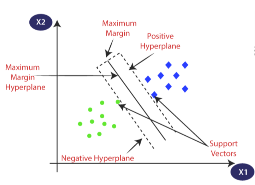
FIGURE 3.1: Schematic Diagram of SVM
All the key elements of the SVM binary classifier is explained in the Figure 3.1.
3.8.12.1 Linear Decision Function
SVM starts with a linear decision function. Given a dataset with feature vectors \(x\) and corresponding labels \(y\) in \(\{-1, 1\}\), the decision function is \(f(x) = w * x + b\), where \(w\) is the weight vector and \(b\) is the bias term. The classification rule is straightforward: if \(f(x) >= 0\), assign the data point to class 1; otherwise, assign it to class -1.
3.8.12.2 Geometric Interpretation
The hyperplane in SVM is chosen to maximize the margin, which is the distance between the hyperplane and the nearest data points from each class. These crucial data points are called support vectors, and the optimization goal is to maximize the margin for a more robust and generalized model.
3.8.13 Optimization Process
3.8.13.1 Objective Function and Lagrangian
To formalize the optimization problem, SVM introduces an objective function that reflects the margin. The goal is to maximize \(M = 2 / ||w||\) subject to the constraint \(y_i(w * x_i + b) >= 1\) for all data points. This is a constrained optimization problem, and we formulate the Lagrangian:
\[\mathcal{L}(w, b, \alpha) = \frac{1}{2}||w||^2 - \sum_{i=1}^{n} \alpha_i [y_i(w * x_i + b) - 1]\]
3.8.13.2 Dual Problem and Optimization
By setting the partial derivatives of the Lagrangian with respect to \(w\) and \(b\) to zero, we derive the dual problem. The solution involves finding the optimal values of Lagrange multipliers (\(alpha\)), which correspond to the support vectors. The decision function becomes \(f(x) = \sum(\alpha_i * y_i * x_i * x) + b\), emphasizing the importance of support vectors in defining the hyperplane.
3.8.14 Non-Linear Extension with Kernels
3.8.14.1 Kernel Trick
SVM’s applicability extends beyond linearly separable data. The kernel trick allows SVM to handle non-linear data by mapping the input space into a higher-dimensional space. The decision function becomes \(f(x) = \sum(\alpha_i * y_i * K(x_i, x)) + b\), where \(K(x_i, x)\) is the kernel function. Common kernels include the linear kernel \(K(x_i, x) = x_i * x\)), polynomial kernel, and radial basis function (RBF) kernel.
3.8.14.2 Soft Margin SVM
In realistic scenarios, data might not be perfectly separable. Soft Margin SVM introduces slack variables to allow for some mis-classification, balancing the trade-off between maximizing the margin and minimizing mis-classification.
3.8.14.3 Multiclass SVM
While SVM was originally designed for binary classification, it can be extended to handle multiple classes using strategies like one-vs-one or one-vs-all.
Example: Design a SVM classifier to classify the samples in the iris dataset into defined classes and use suitable measures for report the performance of the model.
Solution:
The Python code for solving this problem is shown bellow:
# Import required libraries
from sklearn import datasets
from sklearn.model_selection import train_test_split,GridSearchCV
from sklearn.svm import SVC # SVC stands for support vector classifier
from sklearn.metrics import accuracy_score
# Split the dataset into training and testing sets
X_train, X_test, y_train, y_test = train_test_split(iris.data, iris.target, test_size=0.3, random_state=42)# Evaluate the accuracy of the classifier on training
accuracy = accuracy_score(y_train, y_pred)
print('Accuracy:', accuracy)# Use the trained SVM classifier to make predictions on the testing data
y_pred = svm.predict(X_test)# Evaluate the accuracy of the classifier
accuracy = accuracy_score(y_test, y_pred)
print('Accuracy:', accuracy)# Identifying the best parameters
grid = {
'C':[0.01,0.1,1,10],
'kernel' : ["linear","poly","rbf","sigmoid"],
'degree' : [1,3,5,7],
'gamma' : [0.01,1]
}
svm  = SVC ()
svm_cv = GridSearchCV(svm, grid, cv = 5)
svm_cv.fit(X_train,y_train)
print("Best Parameters:",svm_cv.best_params_)
print("Train Score:",svm_cv.best_score_)
print("Test Score:",svm_cv.score(X_test,y_test))# visualize seperation boundaries
svm.fit(X_train, y_train)
import numpy as np
import matplotlib.pyplot as plt
# Create a meshgrid of points to plot the decision boundary
x_min, x_max = X_train[:, 0].min() - 1, X_train[:, 0].max() + 1
y_min, y_max = X_train[:, 1].min() - 1, X_train[:, 1].max() + 1
xx, yy = np.meshgrid(np.arange(x_min, x_max, 0.1),
np.arange(y_min, y_max, 0.1))
Z = svm.predict(np.c_[xx.ravel(), yy.ravel()])
Z = Z.reshape(xx.shape)
# Plot the decision boundary and the training points
plt.contourf(xx, yy, Z, alpha=0.4)
plt.scatter(X_train[:, 0], X_train[:, 1], c=y_train, alpha=0.8)
plt.xlabel('Sepal length')
plt.ylabel('Sepal width')
plt.title('SVM classification on Iris dataset')
plt.show()3.8.15 Ensemble methods in Machine Learning
Ensemble methods in machine learning represent a sophisticated approach to enhancing predictive performance by combining the strengths of multiple models. The core idea is rooted in the concept that the collective knowledge and insights of diverse models can compensate for individual model limitations, leading to more accurate and robust predictions. These methods have gained immense popularity due to their ability to significantly improve both classification and regression tasks.
One prevalent category of ensemble methods is Bagging, which involves training multiple instances of the same base model on different subsets of the training data. This process, known as Bootstrap Aggregating, helps mitigate overfitting and improves the overall stability of the model. Random Forest, a popular algorithm, employs bagging with decision trees as base models, resulting in a robust and accurate predictive model.
Boosting, another key category, focuses on sequentially training weak learners, each emphasizing the misclassified instances of the previous ones. AdaBoost and Gradient Boosting Machines are notable algorithms within this category, emphasizing the importance of learning from mistakes to iteratively improve the model’s predictive power.
Stacking, a more advanced ensemble technique, incorporates diverse base models, and a meta-model is trained to combine their predictions effectively. Stacking leverages the strengths of different algorithms and can yield superior performance compared to individual models. Additionally, voting classifiers/regressors provide a simple yet effective ensemble strategy, making predictions based on the majority vote or average of individual models’ predictions.
Ensemble methods offer several advantages, including increased accuracy, improved generalization, robustness to noisy data, and versatility across various machine learning domains. However, they come with challenges, such as increased computational complexity, potential loss of interpretability, and the necessity of selecting diverse and high-quality base models. Overall, understanding and harnessing the potential of ensemble methods empower machine learning practitioners to build more resilient and powerful models for diverse applications.
3.8.16 Comparison between Regression and Classification Models
A brief comparison of regression and classification models.
| Aspect | Regression Model | Classification Model |
|---|---|---|
| Nature of Target Variable | Continuous numeric value | Categorical (discrete) classes |
| Output Representation | Single numeric value | Class label or category |
| Model Function | Captures relationship with continuous output | Defines decision boundaries for classes |
| Evaluation Metrics | Mean Squared Error (MSE), Mean Absolute Error (MAE), R-squared | Accuracy, Precision, Recall, F1 Score, Confusion Matrix |
| Application | Predicting quantities (e.g., sales, temperature) | Categorizing instances (e.g., spam detection, image recognition) |
| Decision Boundary | Not applicable (continuous output) | Defines regions separating different classes |
| Example | Predicting house prices, stock prices | Classifying emails as spam or non-spam |