2 Education, Age, & Population

2.1 Objects, Vectors, Dataframes, & Tibbles

Fortunately, the U.S. Census Bureau has population, age, and education data all in one spot. As such, we’ll tackle all three of those variables in this single section, starting with where and how to download the data. First, however, let’s take this opportunity to create a convenience object with R. We’ll need to remember the six other states that we’re gathering data for throughout this document. Certainly, we could memorize them or reference the Introduction of this document over and over, but we could also store that information in a memorably named object and have R remember it for us! Then, we can just type the object name into the console and have R remind us which states we’re interested in whenever we need a refresher! In the code below, we create a data.frame object named states_of_interest and tell R to store the full state names and the abbreviations of the six states we need to gather data for inside of of two appropriately named columns. We then tell R to show us the output of the states_of_interest object.

states_of_interest <- data.frame(State = c("Alabama", "Kentucky", "Missouri", "South Carolina", "Texas", "West Virginia"),
                                 Abb = c("AL", "KY", "MO", "SC", "TX", "WV"))
states_of_interest

##            State Abb
## 1        Alabama  AL
## 2       Kentucky  KY
## 3       Missouri  MO
## 4 South Carolina  SC
## 5          Texas  TX
## 6  West Virginia  WV

The reason we do names and abbreviations isn’t just in case we have a major lapse in memory and forget what the abbreviations stand for. It’s also so that I can show you the difference between a vector and a dataframe. It’s useful to think about vectors like a column of data. The object name of the vector would be the column name and the data within the vector would be all of the data points you’d see in the rows beneath that name. Each of the columns in our data frame is a vector then! Telling R to show you a lone vector doesn’t print out to the console like a column, however. The code below and it’s console output show what you get instead.

states_of_interest$Abb

## [1] AL KY MO SC TX WV
## Levels: AL KY MO SC TX WV

Note the usage of the $ operator here. The $ operator allows us to access individual columns from a larger dataframe. So, we provide the object name of a dataframe, then the $ operator, and then the object name of the variable we want to reference. We’ll do this often going forward, so remember this. We’ll talk about ways to circumvent overly frequent usage of the $ operator using tidyverse later in Section 2.4. For now, using the tidyverse function tibble(), we can turn this dataframe into what the tidyverse authors call a “tibble” (Müller and Wickham 2019). Run the code below to see the differences.

states_of_interest <- as_tibble(states_of_interest)

states_of_interest

## # A tibble: 6 x 2
##   State          Abb  
##   <fct>          <fct>
## 1 Alabama        AL   
## 2 Kentucky       KY   
## 3 Missouri       MO   
## 4 South Carolina SC   
## 5 Texas          TX   
## 6 West Virginia  WV

See how this gives us useful information that we didn’t have before? Not only do we get the contents of the dataframe, but we also get the following:

The dimensions of a dataframe, or number of rows by the number of columns, i.e. A tibble: 6x2
The column names, or variable names, contained within, i.e. states_of_interest$State $Abb
The types of the variables, i.e. <fctr>, which stands for “factor.”

There’s nothing wrong per se with the console output we originally had for states_of_interest, but it’s quite minimalistic compared to the tibble() form. Importantly, “tibbles” are dataframes, but they’re also different in a lot of ways. If you’re interested in the nuances between them outside of the few I’ve pointed out here, visit https://tibble.tidyverse.org/. Alternatively, you can run vignette("tibble") and read some useful descriptions of the differences in the comfort of your console!

We’ll also need to remember the variables that we want to collect. Thankfully, we’ve already collected all of them for MS and named our columns accordingly in that dataset. As such, we can simply type the following at any time to have R remind us what variables we’re looking for:

names(MS_Model_Dataset_Reduced_Form)

## [1] "County"                          "WalkerMean.MuniProportion.Multi"
## [3] "WalkerMean.PopProportion.Multi"  "PA.Ratio"                       
## [5] "PercentBachelorOrHigher"         "PercentUnder18"                 
## [7] "AvgAQPM01_14"                    "PrimaryCarePhysRatio"           
## [9] "PercentSmokers"

Now, with some of the terminology and convenience setup out of the way, we can go download some Census data!

2.2 Downloading the Census Education Data

To obtain the data we need, I went to the United States Census Bureau’s American Fact Finder tool and selected Advanced Search. For your convenience, this link will take you directly there (U.S. Census Bureau 2010). Under the Geographies tab, select County then add All Counties within … for each of the states in states_of_interest. To do so, select a state name from the Select a state: dropdown menu, click All Counties within …, and click Add to Your Selection. Repeat this process until you have all All Counties within … for the six states of interest. For the PercentBachelorOrHigher variable data, I opened the Topics dropdown, selected People, then Education, and then “Educational Attainment.” Then, I used the drop down menu on the right hand side of the screen next to Show results from: and selected 2010. The 2010 ACS 5-year estimates dataset is the only available dataset that had estimates for each of the states_of_interest and was therefore selected for download and extraction. Left click the first instance of EDUCATIONAL ATTAINMENT in blue text to the left of 2010 ACS 5-year estimates in the Table, File or Document Title column. This will open up an in-browser viewer for the data. Above the table, you’ll see the word Download in blue text; left click it and tick Use the data before clicking OK. For ease of replication in the rest of this tutorial, I suggest extracting the files to a folder in your working directory called Census Data. The video below details how to perform the entirety of this step, but keep in mind the folder you will extract the files to will be situated differently than mine.

Let’s open up the file we downloaded from the Census called ACS_10_5YR_S1501_with_ann.csv, and start to clean it up some. Use the code below to import the data into R on your machine. Notice the usage of the here() function from the here package (Müller 2017). If you don’t already have the here() package installed, you can run install.packages("here") in the console, and R will take care of that for you automatically! The here() function helps you tell R where to find the files you want it to read more easily by always starting from your R project’s root directory. For more information on the here package and why it’s useful with a dash of humor, see https://github.com/jennybc/here_here. Recall, I suggested extracting the files to a file in your project directory called Census Data. If you did exactly that, the code below will execute without hangup. If you named your folder something else or saved it in a different place, you’ll need to correct that or adjust your code to account for it. We use read.csv() here because we’re, well, reading a .csv file! We surround that with as_tibble() because we want this to print more nicely to our console. If you’re feeling brave, try removing head(), running the code again, and looking at the output. Then, also remove as_tibble(), run the code again, and compare. This is one of the clearest examples of why tibbles are preferred that I have encountered.

library(here)
census_edu <- as_tibble(read.csv(here("Census Data", "ACS_10_5YR_S1501_with_ann.csv"), header = T))

head(census_edu)

## # A tibble: 6 x 231
##   GEO.id GEO.id2 GEO.display.lab~ HC01_EST_VC01 HC01_MOE_VC01 HC02_EST_VC01
##   <fct>  <fct>   <fct>            <fct>         <fct>         <fct>        
## 1 Id     Id2     Geography        Total; Estim~ Total; Margi~ Male; Estima~
## 2 05000~ 01001   Autauga County,~ 4546          112           2254         
## 3 05000~ 01003   Baldwin County,~ 13257         211           6825         
## 4 05000~ 01005   Barbour County,~ 2590          61            1524         
## 5 05000~ 01007   Bibb County, Al~ 2230          329           1298         
## 6 05000~ 01009   Blount County, ~ 4559          99            2315         
## # ... with 225 more variables: HC02_MOE_VC01 <fct>, HC03_EST_VC01 <fct>,
## #   HC03_MOE_VC01 <fct>, HC01_EST_VC02 <fct>, HC01_MOE_VC02 <fct>,
## #   HC02_EST_VC02 <fct>, HC02_MOE_VC02 <fct>, HC03_EST_VC02 <fct>,
## #   HC03_MOE_VC02 <fct>, HC01_EST_VC03 <fct>, HC01_MOE_VC03 <fct>,
## #   HC02_EST_VC03 <fct>, HC02_MOE_VC03 <fct>, HC03_EST_VC03 <fct>,
## #   HC03_MOE_VC03 <fct>, HC01_EST_VC04 <fct>, HC01_MOE_VC04 <fct>,
## #   HC02_EST_VC04 <fct>, HC02_MOE_VC04 <fct>, HC03_EST_VC04 <fct>,
## #   HC03_MOE_VC04 <fct>, HC01_EST_VC05 <fct>, HC01_MOE_VC05 <fct>,
## #   HC02_EST_VC05 <fct>, HC02_MOE_VC05 <fct>, HC03_EST_VC05 <fct>,
## #   HC03_MOE_VC05 <fct>, HC01_EST_VC07 <fct>, HC01_MOE_VC07 <fct>,
## #   HC02_EST_VC07 <fct>, HC02_MOE_VC07 <fct>, HC03_EST_VC07 <fct>,
## #   HC03_MOE_VC07 <fct>, HC01_EST_VC08 <fct>, HC01_MOE_VC08 <fct>,
## #   HC02_EST_VC08 <fct>, HC02_MOE_VC08 <fct>, HC03_EST_VC08 <fct>,
## #   HC03_MOE_VC08 <fct>, HC01_EST_VC09 <fct>, HC01_MOE_VC09 <fct>,
## #   HC02_EST_VC09 <fct>, HC02_MOE_VC09 <fct>, HC03_EST_VC09 <fct>,
## #   HC03_MOE_VC09 <fct>, HC01_EST_VC10 <fct>, HC01_MOE_VC10 <fct>,
## #   HC02_EST_VC10 <fct>, HC02_MOE_VC10 <fct>, HC03_EST_VC10 <fct>,
## #   HC03_MOE_VC10 <fct>, HC01_EST_VC11 <fct>, HC01_MOE_VC11 <fct>,
## #   HC02_EST_VC11 <fct>, HC02_MOE_VC11 <fct>, HC03_EST_VC11 <fct>,
## #   HC03_MOE_VC11 <fct>, HC01_EST_VC12 <fct>, HC01_MOE_VC12 <fct>,
## #   HC02_EST_VC12 <fct>, HC02_MOE_VC12 <fct>, HC03_EST_VC12 <fct>,
## #   HC03_MOE_VC12 <fct>, HC01_EST_VC13 <fct>, HC01_MOE_VC13 <fct>,
## #   HC02_EST_VC13 <fct>, HC02_MOE_VC13 <fct>, HC03_EST_VC13 <fct>,
## #   HC03_MOE_VC13 <fct>, HC01_EST_VC14 <fct>, HC01_MOE_VC14 <fct>,
## #   HC02_EST_VC14 <fct>, HC02_MOE_VC14 <fct>, HC03_EST_VC14 <fct>,
## #   HC03_MOE_VC14 <fct>, HC01_EST_VC16 <fct>, HC01_MOE_VC16 <fct>,
## #   HC02_EST_VC16 <fct>, HC02_MOE_VC16 <fct>, HC03_EST_VC16 <fct>,
## #   HC03_MOE_VC16 <fct>, HC01_EST_VC17 <fct>, HC01_MOE_VC17 <fct>,
## #   HC02_EST_VC17 <fct>, HC02_MOE_VC17 <fct>, HC03_EST_VC17 <fct>,
## #   HC03_MOE_VC17 <fct>, HC01_EST_VC19 <fct>, HC01_MOE_VC19 <fct>,
## #   HC02_EST_VC19 <fct>, HC02_MOE_VC19 <fct>, HC03_EST_VC19 <fct>,
## #   HC03_MOE_VC19 <fct>, HC01_EST_VC20 <fct>, HC01_MOE_VC20 <fct>,
## #   HC02_EST_VC20 <fct>, HC02_MOE_VC20 <fct>, HC03_EST_VC20 <fct>,
## #   HC03_MOE_VC20 <fct>, HC01_EST_VC21 <fct>, ...

I also recommend taking a look at what the data looks like in the data viewer as well. Tibbles are great for glancing at a dataset, but to really get an in-depth feel for what it looks like, the viewer is unmatched. Just use the View() function on objects to open them in the data viewer of RStudio. Note the capital V! Table 2.1 below shows a partial preview of what the data will resemble in the viewer.

Table 2.1: Uncleaned Census Education Data Preview
GEO.id	GEO.id2	GEO.display.label	HC01_EST_VC01	HC01_MOE_VC01	HC02_EST_VC01	HC02_MOE_VC01	HC03_EST_VC01	HC03_MOE_VC01	HC01_EST_VC02	HC01_MOE_VC02	HC02_EST_VC02	HC02_MOE_VC02	HC03_EST_VC02	HC03_MOE_VC02	HC01_EST_VC03	HC01_MOE_VC03	HC02_EST_VC03	HC02_MOE_VC03	HC03_EST_VC03	HC03_MOE_VC03	HC01_EST_VC04	HC01_MOE_VC04	HC02_EST_VC04	HC02_MOE_VC04	HC03_EST_VC04	HC03_MOE_VC04	HC01_EST_VC05	HC01_MOE_VC05	HC02_EST_VC05	HC02_MOE_VC05	HC03_EST_VC05	HC03_MOE_VC05	HC01_EST_VC07	HC01_MOE_VC07	HC02_EST_VC07	HC02_MOE_VC07	HC03_EST_VC07	HC03_MOE_VC07	HC01_EST_VC08	HC01_MOE_VC08	HC02_EST_VC08	HC02_MOE_VC08	HC03_EST_VC08	HC03_MOE_VC08	HC01_EST_VC09	HC01_MOE_VC09	HC02_EST_VC09	HC02_MOE_VC09	HC03_EST_VC09	HC03_MOE_VC09	HC01_EST_VC10	HC01_MOE_VC10	HC02_EST_VC10	HC02_MOE_VC10	HC03_EST_VC10	HC03_MOE_VC10	HC01_EST_VC11	HC01_MOE_VC11	HC02_EST_VC11	HC02_MOE_VC11	HC03_EST_VC11	HC03_MOE_VC11	HC01_EST_VC12	HC01_MOE_VC12	HC02_EST_VC12	HC02_MOE_VC12	HC03_EST_VC12	HC03_MOE_VC12	HC01_EST_VC13	HC01_MOE_VC13	HC02_EST_VC13	HC02_MOE_VC13	HC03_EST_VC13	HC03_MOE_VC13	HC01_EST_VC14	HC01_MOE_VC14	HC02_EST_VC14	HC02_MOE_VC14	HC03_EST_VC14	HC03_MOE_VC14	HC01_EST_VC16	HC01_MOE_VC16	HC02_EST_VC16	HC02_MOE_VC16	HC03_EST_VC16	HC03_MOE_VC16	HC01_EST_VC17	HC01_MOE_VC17	HC02_EST_VC17	HC02_MOE_VC17	HC03_EST_VC17	HC03_MOE_VC17	HC01_EST_VC19	HC01_MOE_VC19	HC02_EST_VC19	HC02_MOE_VC19	HC03_EST_VC19	HC03_MOE_VC19	HC01_EST_VC20	HC01_MOE_VC20	HC02_EST_VC20	HC02_MOE_VC20	HC03_EST_VC20	HC03_MOE_VC20	HC01_EST_VC21	HC01_MOE_VC21	HC02_EST_VC21	HC02_MOE_VC21	HC03_EST_VC21	HC03_MOE_VC21	HC01_EST_VC23	HC01_MOE_VC23	HC02_EST_VC23	HC02_MOE_VC23	HC03_EST_VC23	HC03_MOE_VC23	HC01_EST_VC24	HC01_MOE_VC24	HC02_EST_VC24	HC02_MOE_VC24	HC03_EST_VC24	HC03_MOE_VC24	HC01_EST_VC25	HC01_MOE_VC25	HC02_EST_VC25	HC02_MOE_VC25	HC03_EST_VC25	HC03_MOE_VC25	HC01_EST_VC27	HC01_MOE_VC27	HC02_EST_VC27	HC02_MOE_VC27	HC03_EST_VC27	HC03_MOE_VC27	HC01_EST_VC28	HC01_MOE_VC28	HC02_EST_VC28	HC02_MOE_VC28	HC03_EST_VC28	HC03_MOE_VC28	HC01_EST_VC29	HC01_MOE_VC29	HC02_EST_VC29	HC02_MOE_VC29	HC03_EST_VC29	HC03_MOE_VC29	HC01_EST_VC31	HC01_MOE_VC31	HC02_EST_VC31	HC02_MOE_VC31	HC03_EST_VC31	HC03_MOE_VC31	HC01_EST_VC32	HC01_MOE_VC32	HC02_EST_VC32	HC02_MOE_VC32	HC03_EST_VC32	HC03_MOE_VC32	HC01_EST_VC33	HC01_MOE_VC33	HC02_EST_VC33	HC02_MOE_VC33	HC03_EST_VC33	HC03_MOE_VC33	HC01_EST_VC37	HC01_MOE_VC37	HC02_EST_VC37	HC02_MOE_VC37	HC03_EST_VC37	HC03_MOE_VC37	HC01_EST_VC38	HC01_MOE_VC38	HC02_EST_VC38	HC02_MOE_VC38	HC03_EST_VC38	HC03_MOE_VC38	HC01_EST_VC39	HC01_MOE_VC39	HC02_EST_VC39	HC02_MOE_VC39	HC03_EST_VC39	HC03_MOE_VC39	HC01_EST_VC40	HC01_MOE_VC40	HC02_EST_VC40	HC02_MOE_VC40	HC03_EST_VC40	HC03_MOE_VC40	HC01_EST_VC44	HC01_MOE_VC44	HC02_EST_VC44	HC02_MOE_VC44	HC03_EST_VC44	HC03_MOE_VC44	HC01_EST_VC45	HC01_MOE_VC45	HC02_EST_VC45	HC02_MOE_VC45	HC03_EST_VC45	HC03_MOE_VC45	HC01_EST_VC46	HC01_MOE_VC46	HC02_EST_VC46	HC02_MOE_VC46	HC03_EST_VC46	HC03_MOE_VC46	HC01_EST_VC47	HC01_MOE_VC47	HC02_EST_VC47	HC02_MOE_VC47	HC03_EST_VC47	HC03_MOE_VC47	HC01_EST_VC48	HC01_MOE_VC48	HC02_EST_VC48	HC02_MOE_VC48	HC03_EST_VC48	HC03_MOE_VC48	HC01_EST_VC49	HC01_MOE_VC49	HC02_EST_VC49	HC02_MOE_VC49	HC03_EST_VC49	HC03_MOE_VC49	HC01_EST_VC52	HC01_MOE_VC52	HC02_EST_VC52	HC02_MOE_VC52	HC03_EST_VC52	HC03_MOE_VC52
Id	Id2	Geography	Total; Estimate; Population 18 to 24 years	Total; Margin of Error; Population 18 to 24 years	Male; Estimate; Population 18 to 24 years	Male; Margin of Error; Population 18 to 24 years	Female; Estimate; Population 18 to 24 years	Female; Margin of Error; Population 18 to 24 years	Total; Estimate; Less than high school graduate	Total; Margin of Error; Less than high school graduate	Male; Estimate; Less than high school graduate	Male; Margin of Error; Less than high school graduate	Female; Estimate; Less than high school graduate	Female; Margin of Error; Less than high school graduate	Total; Estimate; High school graduate (includes equivalency)	Total; Margin of Error; High school graduate (includes equivalency)	Male; Estimate; High school graduate (includes equivalency)	Male; Margin of Error; High school graduate (includes equivalency)	Female; Estimate; High school graduate (includes equivalency)	Female; Margin of Error; High school graduate (includes equivalency)	Total; Estimate; Some college or associate’s degree	Total; Margin of Error; Some college or associate’s degree	Male; Estimate; Some college or associate’s degree	Male; Margin of Error; Some college or associate’s degree	Female; Estimate; Some college or associate’s degree	Female; Margin of Error; Some college or associate’s degree	Total; Estimate; Bachelor’s degree or higher	Total; Margin of Error; Bachelor’s degree or higher	Male; Estimate; Bachelor’s degree or higher	Male; Margin of Error; Bachelor’s degree or higher	Female; Estimate; Bachelor’s degree or higher	Female; Margin of Error; Bachelor’s degree or higher	Total; Estimate; Population 25 years and over	Total; Margin of Error; Population 25 years and over	Male; Estimate; Population 25 years and over	Male; Margin of Error; Population 25 years and over	Female; Estimate; Population 25 years and over	Female; Margin of Error; Population 25 years and over	Total; Estimate; Less than 9th grade	Total; Margin of Error; Less than 9th grade	Male; Estimate; Less than 9th grade	Male; Margin of Error; Less than 9th grade	Female; Estimate; Less than 9th grade	Female; Margin of Error; Less than 9th grade	Total; Estimate; 9th to 12th grade, no diploma	Total; Margin of Error; 9th to 12th grade, no diploma	Male; Estimate; 9th to 12th grade, no diploma	Male; Margin of Error; 9th to 12th grade, no diploma	Female; Estimate; 9th to 12th grade, no diploma	Female; Margin of Error; 9th to 12th grade, no diploma	Total; Estimate; High school graduate (includes equivalency)	Total; Margin of Error; High school graduate (includes equivalency)	Male; Estimate; High school graduate (includes equivalency)	Male; Margin of Error; High school graduate (includes equivalency)	Female; Estimate; High school graduate (includes equivalency)	Female; Margin of Error; High school graduate (includes equivalency)	Total; Estimate; Some college, no degree	Total; Margin of Error; Some college, no degree	Male; Estimate; Some college, no degree	Male; Margin of Error; Some college, no degree	Female; Estimate; Some college, no degree	Female; Margin of Error; Some college, no degree	Total; Estimate; Associate’s degree	Total; Margin of Error; Associate’s degree	Male; Estimate; Associate’s degree	Male; Margin of Error; Associate’s degree	Female; Estimate; Associate’s degree	Female; Margin of Error; Associate’s degree	Total; Estimate; Bachelor’s degree	Total; Margin of Error; Bachelor’s degree	Male; Estimate; Bachelor’s degree	Male; Margin of Error; Bachelor’s degree	Female; Estimate; Bachelor’s degree	Female; Margin of Error; Bachelor’s degree	Total; Estimate; Graduate or professional degree	Total; Margin of Error; Graduate or professional degree	Male; Estimate; Graduate or professional degree	Male; Margin of Error; Graduate or professional degree	Female; Estimate; Graduate or professional degree	Female; Margin of Error; Graduate or professional degree	Total; Estimate; Percent high school graduate or higher	Total; Margin of Error; Percent high school graduate or higher	Male; Estimate; Percent high school graduate or higher	Male; Margin of Error; Percent high school graduate or higher	Female; Estimate; Percent high school graduate or higher	Female; Margin of Error; Percent high school graduate or higher	Total; Estimate; Percent bachelor’s degree or higher	Total; Margin of Error; Percent bachelor’s degree or higher	Male; Estimate; Percent bachelor’s degree or higher	Male; Margin of Error; Percent bachelor’s degree or higher	Female; Estimate; Percent bachelor’s degree or higher	Female; Margin of Error; Percent bachelor’s degree or higher	Total; Estimate; Population 25 to 34 years	Total; Margin of Error; Population 25 to 34 years	Male; Estimate; Population 25 to 34 years	Male; Margin of Error; Population 25 to 34 years	Female; Estimate; Population 25 to 34 years	Female; Margin of Error; Population 25 to 34 years	Total; Estimate; High school graduate or higher	Total; Margin of Error; High school graduate or higher	Male; Estimate; High school graduate or higher	Male; Margin of Error; High school graduate or higher	Female; Estimate; High school graduate or higher	Female; Margin of Error; High school graduate or higher	Total; Estimate; Bachelor’s degree or higher	Total; Margin of Error; Bachelor’s degree or higher	Male; Estimate; Bachelor’s degree or higher	Male; Margin of Error; Bachelor’s degree or higher	Female; Estimate; Bachelor’s degree or higher	Female; Margin of Error; Bachelor’s degree or higher	Total; Estimate; Population 35 to 44 years	Total; Margin of Error; Population 35 to 44 years	Male; Estimate; Population 35 to 44 years	Male; Margin of Error; Population 35 to 44 years	Female; Estimate; Population 35 to 44 years	Female; Margin of Error; Population 35 to 44 years	Total; Estimate; High school graduate or higher	Total; Margin of Error; High school graduate or higher	Male; Estimate; High school graduate or higher	Male; Margin of Error; High school graduate or higher	Female; Estimate; High school graduate or higher	Female; Margin of Error; High school graduate or higher	Total; Estimate; Bachelor’s degree or higher	Total; Margin of Error; Bachelor’s degree or higher	Male; Estimate; Bachelor’s degree or higher	Male; Margin of Error; Bachelor’s degree or higher	Female; Estimate; Bachelor’s degree or higher	Female; Margin of Error; Bachelor’s degree or higher	Total; Estimate; Population 45 to 64 years	Total; Margin of Error; Population 45 to 64 years	Male; Estimate; Population 45 to 64 years	Male; Margin of Error; Population 45 to 64 years	Female; Estimate; Population 45 to 64 years	Female; Margin of Error; Population 45 to 64 years	Total; Estimate; High school graduate or higher	Total; Margin of Error; High school graduate or higher	Male; Estimate; High school graduate or higher	Male; Margin of Error; High school graduate or higher	Female; Estimate; High school graduate or higher	Female; Margin of Error; High school graduate or higher	Total; Estimate; Bachelor’s degree or higher	Total; Margin of Error; Bachelor’s degree or higher	Male; Estimate; Bachelor’s degree or higher	Male; Margin of Error; Bachelor’s degree or higher	Female; Estimate; Bachelor’s degree or higher	Female; Margin of Error; Bachelor’s degree or higher	Total; Estimate; Population 65 years and over	Total; Margin of Error; Population 65 years and over	Male; Estimate; Population 65 years and over	Male; Margin of Error; Population 65 years and over	Female; Estimate; Population 65 years and over	Female; Margin of Error; Population 65 years and over	Total; Estimate; High school graduate or higher	Total; Margin of Error; High school graduate or higher	Male; Estimate; High school graduate or higher	Male; Margin of Error; High school graduate or higher	Female; Estimate; High school graduate or higher	Female; Margin of Error; High school graduate or higher	Total; Estimate; Bachelor’s degree or higher	Total; Margin of Error; Bachelor’s degree or higher	Male; Estimate; Bachelor’s degree or higher	Male; Margin of Error; Bachelor’s degree or higher	Female; Estimate; Bachelor’s degree or higher	Female; Margin of Error; Bachelor’s degree or higher	Total; Estimate; POVERTY RATE FOR THE POPULATION 25 YEARS AND OVER FOR WHOM POVERTY STATUS IS DETERMINED BY EDUCATIONAL ATTAINMENT LEVEL - Less than high school graduate	Total; Margin of Error; POVERTY RATE FOR THE POPULATION 25 YEARS AND OVER FOR WHOM POVERTY STATUS IS DETERMINED BY EDUCATIONAL ATTAINMENT LEVEL - Less than high school graduate	Male; Estimate; POVERTY RATE FOR THE POPULATION 25 YEARS AND OVER FOR WHOM POVERTY STATUS IS DETERMINED BY EDUCATIONAL ATTAINMENT LEVEL - Less than high school graduate	Male; Margin of Error; POVERTY RATE FOR THE POPULATION 25 YEARS AND OVER FOR WHOM POVERTY STATUS IS DETERMINED BY EDUCATIONAL ATTAINMENT LEVEL - Less than high school graduate	Female; Estimate; POVERTY RATE FOR THE POPULATION 25 YEARS AND OVER FOR WHOM POVERTY STATUS IS DETERMINED BY EDUCATIONAL ATTAINMENT LEVEL - Less than high school graduate	Female; Margin of Error; POVERTY RATE FOR THE POPULATION 25 YEARS AND OVER FOR WHOM POVERTY STATUS IS DETERMINED BY EDUCATIONAL ATTAINMENT LEVEL - Less than high school graduate	Total; Estimate; POVERTY RATE FOR THE POPULATION 25 YEARS AND OVER FOR WHOM POVERTY STATUS IS DETERMINED BY EDUCATIONAL ATTAINMENT LEVEL - High school graduate (includes equivalency)	Total; Margin of Error; POVERTY RATE FOR THE POPULATION 25 YEARS AND OVER FOR WHOM POVERTY STATUS IS DETERMINED BY EDUCATIONAL ATTAINMENT LEVEL - High school graduate (includes equivalency)	Male; Estimate; POVERTY RATE FOR THE POPULATION 25 YEARS AND OVER FOR WHOM POVERTY STATUS IS DETERMINED BY EDUCATIONAL ATTAINMENT LEVEL - High school graduate (includes equivalency)	Male; Margin of Error; POVERTY RATE FOR THE POPULATION 25 YEARS AND OVER FOR WHOM POVERTY STATUS IS DETERMINED BY EDUCATIONAL ATTAINMENT LEVEL - High school graduate (includes equivalency)	Female; Estimate; POVERTY RATE FOR THE POPULATION 25 YEARS AND OVER FOR WHOM POVERTY STATUS IS DETERMINED BY EDUCATIONAL ATTAINMENT LEVEL - High school graduate (includes equivalency)	Female; Margin of Error; POVERTY RATE FOR THE POPULATION 25 YEARS AND OVER FOR WHOM POVERTY STATUS IS DETERMINED BY EDUCATIONAL ATTAINMENT LEVEL - High school graduate (includes equivalency)	Total; Estimate; POVERTY RATE FOR THE POPULATION 25 YEARS AND OVER FOR WHOM POVERTY STATUS IS DETERMINED BY EDUCATIONAL ATTAINMENT LEVEL - Some college or associate’s degree	Total; Margin of Error; POVERTY RATE FOR THE POPULATION 25 YEARS AND OVER FOR WHOM POVERTY STATUS IS DETERMINED BY EDUCATIONAL ATTAINMENT LEVEL - Some college or associate’s degree	Male; Estimate; POVERTY RATE FOR THE POPULATION 25 YEARS AND OVER FOR WHOM POVERTY STATUS IS DETERMINED BY EDUCATIONAL ATTAINMENT LEVEL - Some college or associate’s degree	Male; Margin of Error; POVERTY RATE FOR THE POPULATION 25 YEARS AND OVER FOR WHOM POVERTY STATUS IS DETERMINED BY EDUCATIONAL ATTAINMENT LEVEL - Some college or associate’s degree	Female; Estimate; POVERTY RATE FOR THE POPULATION 25 YEARS AND OVER FOR WHOM POVERTY STATUS IS DETERMINED BY EDUCATIONAL ATTAINMENT LEVEL - Some college or associate’s degree	Female; Margin of Error; POVERTY RATE FOR THE POPULATION 25 YEARS AND OVER FOR WHOM POVERTY STATUS IS DETERMINED BY EDUCATIONAL ATTAINMENT LEVEL - Some college or associate’s degree	Total; Estimate; POVERTY RATE FOR THE POPULATION 25 YEARS AND OVER FOR WHOM POVERTY STATUS IS DETERMINED BY EDUCATIONAL ATTAINMENT LEVEL - Bachelor’s degree or higher	Total; Margin of Error; POVERTY RATE FOR THE POPULATION 25 YEARS AND OVER FOR WHOM POVERTY STATUS IS DETERMINED BY EDUCATIONAL ATTAINMENT LEVEL - Bachelor’s degree or higher	Male; Estimate; POVERTY RATE FOR THE POPULATION 25 YEARS AND OVER FOR WHOM POVERTY STATUS IS DETERMINED BY EDUCATIONAL ATTAINMENT LEVEL - Bachelor’s degree or higher	Male; Margin of Error; POVERTY RATE FOR THE POPULATION 25 YEARS AND OVER FOR WHOM POVERTY STATUS IS DETERMINED BY EDUCATIONAL ATTAINMENT LEVEL - Bachelor’s degree or higher	Female; Estimate; POVERTY RATE FOR THE POPULATION 25 YEARS AND OVER FOR WHOM POVERTY STATUS IS DETERMINED BY EDUCATIONAL ATTAINMENT LEVEL - Bachelor’s degree or higher	Female; Margin of Error; POVERTY RATE FOR THE POPULATION 25 YEARS AND OVER FOR WHOM POVERTY STATUS IS DETERMINED BY EDUCATIONAL ATTAINMENT LEVEL - Bachelor’s degree or higher	Total; Estimate; MEDIAN EARNINGS IN THE PAST 12 MONTHS (IN 2010 INFLATION-ADJUSTED DOLLARS) - Population 25 years and over with earnings	Total; Margin of Error; MEDIAN EARNINGS IN THE PAST 12 MONTHS (IN 2010 INFLATION-ADJUSTED DOLLARS) - Population 25 years and over with earnings	Male; Estimate; MEDIAN EARNINGS IN THE PAST 12 MONTHS (IN 2010 INFLATION-ADJUSTED DOLLARS) - Population 25 years and over with earnings	Male; Margin of Error; MEDIAN EARNINGS IN THE PAST 12 MONTHS (IN 2010 INFLATION-ADJUSTED DOLLARS) - Population 25 years and over with earnings	Female; Estimate; MEDIAN EARNINGS IN THE PAST 12 MONTHS (IN 2010 INFLATION-ADJUSTED DOLLARS) - Population 25 years and over with earnings	Female; Margin of Error; MEDIAN EARNINGS IN THE PAST 12 MONTHS (IN 2010 INFLATION-ADJUSTED DOLLARS) - Population 25 years and over with earnings	Total; Estimate; MEDIAN EARNINGS IN THE PAST 12 MONTHS (IN 2010 INFLATION-ADJUSTED DOLLARS) - Less than high school graduate	Total; Margin of Error; MEDIAN EARNINGS IN THE PAST 12 MONTHS (IN 2010 INFLATION-ADJUSTED DOLLARS) - Less than high school graduate	Male; Estimate; MEDIAN EARNINGS IN THE PAST 12 MONTHS (IN 2010 INFLATION-ADJUSTED DOLLARS) - Less than high school graduate	Male; Margin of Error; MEDIAN EARNINGS IN THE PAST 12 MONTHS (IN 2010 INFLATION-ADJUSTED DOLLARS) - Less than high school graduate	Female; Estimate; MEDIAN EARNINGS IN THE PAST 12 MONTHS (IN 2010 INFLATION-ADJUSTED DOLLARS) - Less than high school graduate	Female; Margin of Error; MEDIAN EARNINGS IN THE PAST 12 MONTHS (IN 2010 INFLATION-ADJUSTED DOLLARS) - Less than high school graduate	Total; Estimate; MEDIAN EARNINGS IN THE PAST 12 MONTHS (IN 2010 INFLATION-ADJUSTED DOLLARS) - High school graduate (includes equivalency)	Total; Margin of Error; MEDIAN EARNINGS IN THE PAST 12 MONTHS (IN 2010 INFLATION-ADJUSTED DOLLARS) - High school graduate (includes equivalency)	Male; Estimate; MEDIAN EARNINGS IN THE PAST 12 MONTHS (IN 2010 INFLATION-ADJUSTED DOLLARS) - High school graduate (includes equivalency)	Male; Margin of Error; MEDIAN EARNINGS IN THE PAST 12 MONTHS (IN 2010 INFLATION-ADJUSTED DOLLARS) - High school graduate (includes equivalency)	Female; Estimate; MEDIAN EARNINGS IN THE PAST 12 MONTHS (IN 2010 INFLATION-ADJUSTED DOLLARS) - High school graduate (includes equivalency)	Female; Margin of Error; MEDIAN EARNINGS IN THE PAST 12 MONTHS (IN 2010 INFLATION-ADJUSTED DOLLARS) - High school graduate (includes equivalency)	Total; Estimate; MEDIAN EARNINGS IN THE PAST 12 MONTHS (IN 2010 INFLATION-ADJUSTED DOLLARS) - Some college or associate’s degree	Total; Margin of Error; MEDIAN EARNINGS IN THE PAST 12 MONTHS (IN 2010 INFLATION-ADJUSTED DOLLARS) - Some college or associate’s degree	Male; Estimate; MEDIAN EARNINGS IN THE PAST 12 MONTHS (IN 2010 INFLATION-ADJUSTED DOLLARS) - Some college or associate’s degree	Male; Margin of Error; MEDIAN EARNINGS IN THE PAST 12 MONTHS (IN 2010 INFLATION-ADJUSTED DOLLARS) - Some college or associate’s degree	Female; Estimate; MEDIAN EARNINGS IN THE PAST 12 MONTHS (IN 2010 INFLATION-ADJUSTED DOLLARS) - Some college or associate’s degree	Female; Margin of Error; MEDIAN EARNINGS IN THE PAST 12 MONTHS (IN 2010 INFLATION-ADJUSTED DOLLARS) - Some college or associate’s degree	Total; Estimate; MEDIAN EARNINGS IN THE PAST 12 MONTHS (IN 2010 INFLATION-ADJUSTED DOLLARS) - Bachelor’s degree	Total; Margin of Error; MEDIAN EARNINGS IN THE PAST 12 MONTHS (IN 2010 INFLATION-ADJUSTED DOLLARS) - Bachelor’s degree	Male; Estimate; MEDIAN EARNINGS IN THE PAST 12 MONTHS (IN 2010 INFLATION-ADJUSTED DOLLARS) - Bachelor’s degree	Male; Margin of Error; MEDIAN EARNINGS IN THE PAST 12 MONTHS (IN 2010 INFLATION-ADJUSTED DOLLARS) - Bachelor’s degree	Female; Estimate; MEDIAN EARNINGS IN THE PAST 12 MONTHS (IN 2010 INFLATION-ADJUSTED DOLLARS) - Bachelor’s degree	Female; Margin of Error; MEDIAN EARNINGS IN THE PAST 12 MONTHS (IN 2010 INFLATION-ADJUSTED DOLLARS) - Bachelor’s degree	Total; Estimate; MEDIAN EARNINGS IN THE PAST 12 MONTHS (IN 2010 INFLATION-ADJUSTED DOLLARS) - Graduate or professional degree	Total; Margin of Error; MEDIAN EARNINGS IN THE PAST 12 MONTHS (IN 2010 INFLATION-ADJUSTED DOLLARS) - Graduate or professional degree	Male; Estimate; MEDIAN EARNINGS IN THE PAST 12 MONTHS (IN 2010 INFLATION-ADJUSTED DOLLARS) - Graduate or professional degree	Male; Margin of Error; MEDIAN EARNINGS IN THE PAST 12 MONTHS (IN 2010 INFLATION-ADJUSTED DOLLARS) - Graduate or professional degree	Female; Estimate; MEDIAN EARNINGS IN THE PAST 12 MONTHS (IN 2010 INFLATION-ADJUSTED DOLLARS) - Graduate or professional degree	Female; Margin of Error; MEDIAN EARNINGS IN THE PAST 12 MONTHS (IN 2010 INFLATION-ADJUSTED DOLLARS) - Graduate or professional degree	Total; Estimate; PERCENT IMPUTED - Educational attainment	Total; Margin of Error; PERCENT IMPUTED - Educational attainment	Male; Estimate; PERCENT IMPUTED - Educational attainment	Male; Margin of Error; PERCENT IMPUTED - Educational attainment	Female; Estimate; PERCENT IMPUTED - Educational attainment	Female; Margin of Error; PERCENT IMPUTED - Educational attainment
0500000US01001	01001	Autauga County, Alabama	4546	112	2254	70	2292	91	23.3	4.7	28.6	7.5	18.2	5.4	33.0	4.8	37.7	7.4	28.4	6.6	37.2	5.8	30.4	7.0	43.8	8.4	6.4	2.6	3.2	2.3	9.6	4.7	33884	112	16047	80	17837	104	4.9	0.8	5.1	1.2	4.8	1.3	9.7	1.0	9.4	1.4	10.1	1.2	35.2	2.0	34.4	2.5	36.0	2.6	21.9	1.7	22.6	2.4	21.3	2.0	6.5	0.9	5.0	1.2	7.7	1.3	14.7	1.2	15.3	1.7	14.1	1.6	7.1	0.8	8.2	1.2	6.0	1.0	85.3	1.4	85.5	1.8	85.2	1.6	21.7	1.3	23.5	2.0	20.2	1.7	6370	135	3064	77	3306	92	87.5	3.4	86.3	5.3	88.5	3.7	22.3	4.0	19.5	5.0	24.9	4.9	8269	117	3975	58	4294	85	89.2	2.5	88.7	2.9	89.6	3.3	23.9	3.2	26.2	4.5	21.8	3.7	13185	121	6442	77	6743	89	86.8	1.8	85.7	2.8	87.8	2.1	24.1	2.2	25.7	3.1	22.6	2.8	6060	66	2566	29	3494	67	74.7	3.3	79.3	4.2	71.3	4.4	13.0	2.8	18.6	4.5	8.8	2.6	23.7	5.5	20.2	6.5	26.9	6.9	8.4	1.8	6.5	2.2	9.9	2.5	4.9	1.6	3.0	1.7	6.5	2.2	2.4	1.2	1.9	1.4	3.0	1.6	34167	1533	44112	1824	26832	915	19643	4768	27439	2824	13994	1703	29010	1559	36257	3441	22441	2081	33552	2830	46871	3264	26403	1187	49699	4891	64635	4384	40800	2711	56389	4927	72662	7188	42891	6239	2.0
0500000US01003	01003	Baldwin County, Alabama	13257	211	6825	82	6432	193	21.0	3.0	25.3	4.0	16.3	4.2	37.3	4.0	40.4	5.0	33.9	5.4	34.9	3.4	28.4	4.1	41.9	4.8	6.9	1.9	5.9	2.4	7.9	2.3	121560	210	58269	88	63291	189	3.9	0.5	4.3	0.7	3.5	0.6	8.5	0.5	9.5	0.9	7.7	0.6	29.9	1.0	29.4	1.3	30.4	1.3	23.2	0.9	22.3	1.1	24.1	1.3	7.6	0.5	5.9	0.7	9.2	0.8	18.1	0.8	19.8	1.2	16.6	1.0	8.7	0.6	8.9	0.8	8.5	0.7	87.6	0.6	86.2	1.1	88.8	0.8	26.8	1.0	28.7	1.3	25.1	1.1	19930	205	9911	72	10019	193	87.7	2.0	85.5	2.4	89.8	2.6	25.7	2.8	21.1	2.9	30.2	3.9	23424	200	11444	79	11980	171	89.3	1.6	87.0	2.2	91.6	2.2	28.5	2.2	26.3	2.9	30.7	2.9	49216	203	23471	82	25745	202	88.9	1.0	86.3	1.5	91.2	1.3	28.3	1.4	31.4	2.1	25.5	1.8	28990	115	13443	73	15547	87	83.9	1.3	86.0	1.8	82.1	2.0	23.7	1.7	31.6	2.5	16.9	2.2	22.5	3.2	20.0	3.7	25.3	4.4	11.3	1.5	6.4	1.4	15.5	2.2	6.3	1.1	4.9	1.2	7.4	1.6	2.7	0.8	2.1	0.8	3.4	1.1	30780	832	40044	1089	23118	874	18332	1748	22147	2053	12208	2983	25201	1327	32365	1627	18932	1396	29639	1144	39988	1960	22765	1195	45147	2485	59914	4623	35791	1576	51478	1667	73986	9777	45025	3921	3.5
0500000US01005	01005	Barbour County, Alabama	2590	61	1524	44	1066	41	32.3	7.0	35.7	10.6	27.4	7.9	43.7	6.9	44.4	9.4	42.9	10.3	23.1	5.5	18.7	5.9	29.4	10.7	0.9	0.7	1.2	1.1	0.4	0.6	18879	68	9942	50	8937	51	9.0	1.1	8.5	1.4	9.5	1.7	19.2	1.8	21.0	2.4	17.2	2.3	35.4	2.4	36.1	2.7	34.6	3.1	16.0	1.7	16.6	2.7	15.3	1.9	7.0	1.0	5.2	1.3	9.0	1.6	7.5	1.1	6.9	1.5	8.2	1.7	6.0	1.2	5.7	1.2	6.3	1.7	71.9	1.9	70.5	2.4	73.4	2.6	13.5	1.7	12.6	2.0	14.5	2.1	3748	82	2267	56	1481	57	72.8	4.4	67.7	5.1	80.6	8.1	8.9	3.2	6.0	3.5	13.4	5.6	3840	69	2243	67	1597	30	78.3	4.1	75.8	5.5	81.7	6.9	14.2	4.0	7.0	3.4	24.2	7.6	7485	57	3825	46	3660	35	74.4	3.1	72.9	3.3	75.9	4.3	15.0	2.6	17.3	3.5	12.7	2.9	3806	45	1607	26	2199	21	59.5	4.0	61.3	5.5	58.2	5.3	14.4	3.1	18.8	5.2	11.2	3.0	39.4	5.9	32.9	8.0	44.6	6.3	20.4	4.2	15.6	5.0	24.9	5.4	13.1	4.0	5.4	3.4	19.3	5.6	2.4	1.3	0.8	1.1	3.9	2.3	22508	1498	26424	2550	20269	1649	13129	2803	13011	5732	13221	2826	21611	2372	26639	3562	17887	1849	24197	2460	31739	9078	21112	2004	39428	4454	45179	10026	33984	6737	47930	6079	52321	12791	46250	5114	4.8
0500000US01007	01007	Bibb County, Alabama	2230	329	1298	329	932	*****	26.6	8.9	39.5	15.9	8.7	7.8	41.7	12.0	47.2	16.6	34.0	12.5	28.7	8.4	10.6	8.4	53.8	13.4	3.0	2.8	2.6	4.2	3.5	3.5	15082	329	7911	329	7171	*****	9.8	2.5	10.4	3.9	9.0	2.6	15.7	3.0	16.6	4.1	14.7	3.5	42.3	3.5	43.7	4.1	40.8	4.9	16.9	2.4	13.4	3.2	20.6	3.3	5.4	1.4	5.6	1.8	5.1	2.1	7.5	1.8	8.4	2.4	6.5	2.4	2.6	0.9	1.8	0.8	3.3	1.4	74.5	3.6	73.0	4.9	76.3	4.3	10.0	2.1	10.2	2.7	9.8	2.7	2754	320	1463	320	1291	*****	82.2	8.3	80.2	10.4	84.4	10.9	13.1	6.0	10.9	4.7	15.6	10.6	3604	333	2113	333	1491	*****	83.0	5.9	79.7	8.1	87.7	6.6	10.6	4.7	10.0	6.5	11.3	5.3	5912	*****	3151	*****	2761	*****	72.2	5.4	70.1	6.9	74.6	6.9	8.5	2.8	8.3	3.8	8.9	3.2	2812	*****	1184	*****	1628	*****	61.1	6.2	59.6	10.3	62.2	7.6	9.4	3.9	14.9	6.6	5.5	3.4	20.4	5.6	17.5	6.1	24.0	8.6	10.3	3.5	8.3	4.6	12.5	4.9	3.3	1.7	2.0	1.6	4.3	3.0	2.7	3.1	3.5	5.3	1.8	3.2	31657	2027	38414	3611	20564	1719	31065	5731	34291	7154	13793	7836	28054	2819	33213	3321	19598	4493	32147	7486	42331	6274	19872	3997	53980	11334	67656	32600	36779	14679	49896	8646	48229	28793	51563	13171	5.1
0500000US01009	01009	Blount County, Alabama	4559	99	2315	48	2244	74	22.4	4.6	26.3	7.1	18.3	5.9	39.0	6.5	41.0	8.6	36.9	7.9	37.6	6.1	30.8	7.1	44.6	8.4	1.0	0.9	1.8	1.6	0.3	0.4	38085	107	18447	112	19638	126	9.4	1.0	9.9	1.4	8.9	1.3	15.9	1.3	16.0	1.9	15.8	1.9	36.4	1.8	37.1	2.6	35.8	2.1	19.5	1.4	19.5	2.2	19.4	1.7	6.2	0.8	4.6	0.9	7.7	1.2	8.4	1.0	9.0	1.4	7.7	1.3	4.2	0.7	3.8	1.0	4.5	0.9	74.7	1.6	74.1	2.3	75.2	2.2	12.5	1.4	12.8	1.7	12.2	1.7	6932	181	3544	73	3388	173	74.2	4.1	70.5	6.4	78.1	6.1	11.8	2.4	13.0	3.9	10.5	3.0	8080	175	4110	107	3970	132	80.3	3.4	80.0	4.3	80.6	4.6	14.3	3.1	11.8	3.2	16.9	4.4	15019	193	7290	107	7729	168	77.5	2.4	76.5	3.3	78.4	3.0	14.0	2.3	15.3	3.1	12.9	2.5	8054	132	3503	69	4551	93	64.1	3.6	65.5	5.3	63.0	4.3	8.5	2.0	8.8	2.7	8.3	2.9	22.6	3.3	17.3	3.8	27.9	5.3	11.1	2.0	9.4	2.7	12.8	2.6	4.6	1.2	2.5	1.1	6.3	1.9	4.0	2.1	2.6	1.9	5.4	4.0	31435	809	37199	1647	24488	2151	22819	2544	27086	2116	15767	2692	27791	2635	36710	2418	19234	1722	33684	2094	43392	2141	28688	2179	42208	2855	45506	3342	37179	7687	53730	1997	59660	21417	51587	1865	4.8

If you scrolled far enough across you saw that, clearly, this data needs a lot of work to be even remotely in line with what we need from it. There are a lot of columns, and the first row contains variable descriptions rather than actual county data. Time to show off dplyr from the tidyverse in the proceeding sections (Wickham et al. 2019).

2.3 The “Pipe” Operator

First of all, the magrittr package included in the tidyverse gives us the %>% operator, also referred to as the “pipe” operator (Bache and Wickham 2014). The %>% operator is extremely useful because it allows us to write code in a way that is easier to read after the fact, and it saves us typing the same object name repetitively. Take the code below, for example. Notice how the %>% operator is at the end of each line of code besides the last? When “piping” we present an object name followed by the %>% operator, present operations we’d like R to perform on the provided object name on the next line, include the %>% operator at the end of that line, present more operations to be done on the next line, and so on. Note that while you don’t technically have to break pipe operations across multiple lines, doing so is a best practice that will make your code much easier to follow both for yourself and potential future readers, hence why I recommend it here. Many R functions take the object name of the data you want that function to operate on as their first argument. The %>% operator lets you circumvent having to type that object name as the first argument over and over.

If we wrote, for example,

foo %>%
  ... %>%
  ... %>%
  ...

we could think of this as a plain English sentence that would read, “Take foo, then …, then …, then …” The final product would be whatever is left of foo after all of those operations had been done in sequential order from top to bottom. Note, it’s not required that you insert a line break after each pipe, but doing so is a common practice that will improve the readability of your code.

2.4 Cleaning the Census Education Data

With the basics of “piping” introduced, let’s turn to some of the functions available with the dplyr package from the tidyverse that make cleaning and tidying data more intuitive.

I break this first cleaning example into two sections. First, in Section 2.4.1 I’ll show you an easy way to select columns through some manual inspection of the data and a couple lines of code. In Section 2.4.2, I’ll introduce some more advanced ways you could do the same selection without needing to do as much manual inspection of the data by taking advantage of additional R functions.

2.4.1 Selection via Manual Inspection

Below, we tell R to create a new object named census_edu_clean that is the result of piping census_edu through a series of operations. The first function, or verb, we use to do those operations is select(). You can always type a question mark followed by any function name in the console to read the documentation of a function. Try ?select, for example.

Use select() when you want to select certain columns to keep from a dataset. You can supply select() with either the column number or the column name of the columns you’d like to keep. If you want to keep multiple columns, which you often will, you simply separate each consecutive desired column number or name with a comma.

This step is where we’ll need to do some manual inspection to find the column names we are interested in. In this instance, we’re interested in the county names and the percentage of the county population with a bachelor’s degree or higher. Again, by looking closely at the Census education data by using the previously mentioned View() function, we can see the data includes indecipherable shorthand for the column names and a description of the data inside each column in the first row. Actual data doesn’t begin until the second row. We can identify the contents of a column by scrolling across the viewer and reading the entry in the first row for each column. Once we’ve identified the column we want, we can supply its column name to select() to tell R that’s the one we’d like to keep.

Scrolling across the first row, we can quickly see that Geo.display.label is the column name for Geography, so we know we need to supply that to select() down the line. You might also realize that there appears to be a noticeable pattern for how the later columns are ordered. Generally, the description of what was measured proceeds the second semicolon. For each measurement, the following pattern exists: Total; Estimate; … then Total; Margin of Error; … then Male; Estimate; … then Male; Margin of Error; … then Female; Estimate; … then Female; Margin of Error; …. We know right away that we’re only interested in the Total; Estimate; … column for whatever measurement description most nearly matches “bachelor’s degree or higher.” If you continue scrolling across, you’ll notice there’s a column that matches that exact pattern: Total; Estimate; Bachelor’s degree or higher. Seeing that, remember its associated column name, HC01_EST_VC05, because that’s the second column name we need to supply the select() function with.

Helpfully, you can rename columns within the select() function as you select them. Since the column names that already exist are uninformative, let’s replace them with more easily understood substitutes, County and PercentBachelorOrHigher respectively, by typing the new name we want followed by an equal sign and the old name.

This code illustrates how you would perform what we’ve discussed above, and Table 2.2 presents a preview of the output created through this usage of select().

View(census_edu)

census_edu_clean <- census_edu %>%
  select(County = GEO.display.label, PercentBachelorOrHigher = HC01_EST_VC05)

Table 2.2: Preview of Manually Selected Columns
County	PercentBachelorOrHigher
Geography	Total; Estimate; Bachelor’s degree or higher
Autauga County, Alabama	6.4
Baldwin County, Alabama	6.9
Barbour County, Alabama	0.9
Bibb County, Alabama	3.0
Blount County, Alabama	1.0

2.4.2 Selection via Conditions & Additional Cleaning

As you’ve seen in Section 2.4.1, you would normally feed the column names or column numbers that you wanted to keep to the select() function. I do that below in a slightly more advanced way. Again, our Census data is somewhat strange in that we have the column names followed by a description of what the column name stands for in the first row. The second row and beyond is where the actual data begins. Sometimes manual inspection is easy enough and can get you the column numbers or column names that you’re interested in without much hassle. Other times, there are an overly burdensome number of columns for any individual to manually read through. Below, I discuss how you could perform the same selection as we did in Section 2.4.1 with conditional arguments passed to the select() function that will find the column numbers you want for you. I’ll also demonstrate some of the pitfalls of manual inspection via example.

Since we’re only interested in the percentage of the total population with a bachelor’s degree or higher, I tell R I want it to keep only columns that contain the strings “Geography” or “Total; Estimate; Bachelor’s degree or higher” in the first row using the str_detect() function. Assume for a moment we hadn’t done the full extent of manual inspection that we did earlier. We still know to keep “Geography” because that contains our county and state names. We can test “Total; Estimate; Bachelor’s degree or higher” because we’ve done enough manual inspection to identify the "Total; Estimate; … pattern, and since we know we know the first letter of each word following a semicolon is capitalized, we can supply a reasonable guess as to what the measurement we’re looking for is named, “Bachelor’s degree or higher”.

To test where these strings are, however, I need index positions. Index positions are ways to access subsets of information inside of R objects. You reference them by proceeding an object name with brackets[] and inserting positions within those brackets. Said positions generally consist of two numbers separated by a comma, though you can use vectors separated by commas as well. The first number is row number, and the second number is the column number. So, [1,1] would reference the observation in the first row of the first column of some object. If you omit a number on the left of the comma, that translates to all rows. If you omit a number on the right of the comma, that stands for all columns. For example, [1,] means all values in row one across all columns. If, instead, you were to write [,1], that would translate to all values in all rows of column one. For more detailed explanations of how to reference index positions of R objects, see the tutorials mentioned at the beginning of this document.

Thankfully, the which() function returns index positions as its output. The str_detect() function from the tidyverse package stringr will tell you which values inside of a vector contain a string pattern and which don’t (Wickham 2019). Since we only want those that do math the supplied pattern, we tell which() to look for where str_detect() is true, i.e. == T. To get a vector from a row, we must use unlist(). We can use . as a placeholder for the object name we’re piping where needed, hence .[1,] in the unlist() argument. Typically, when you want to reference a part of a the piped object via indexing, you’ll need to use the . as a placeholder for the objectname before adding the bracketed index positions.

Putting all of this together, you can come up with the lines of code below. Running these lines may supply you with an unexpected result, however.

census_edu_clean <- census_edu %>%
  select(County = which(str_detect(unlist(.[1,]), "Geography") == T), PercentBachelorOrHigher = which(str_detect(unlist(.[1,]), "Total; Estimate; Bachelor's degree or higher") == T))

Table 2.3: Example of Multiple Columns Matching a Condition
County	PercentBachelorOrHigher1	PercentBachelorOrHigher2	PercentBachelorOrHigher3	PercentBachelorOrHigher4	PercentBachelorOrHigher5
Geography	Total; Estimate; Bachelor’s degree or higher	Total; Estimate; Bachelor’s degree or higher	Total; Estimate; Bachelor’s degree or higher	Total; Estimate; Bachelor’s degree or higher	Total; Estimate; Bachelor’s degree or higher
Autauga County, Alabama	6.4	22.3	23.9	24.1	13.0
Baldwin County, Alabama	6.9	25.7	28.5	28.3	23.7
Barbour County, Alabama	0.9	8.9	14.2	15.0	14.4
Bibb County, Alabama	3.0	13.1	10.6	8.5	9.4
Blount County, Alabama	1.0	11.8	14.3	14.0	8.5

The code above returned several columns rather than a single column named PercentBachelorOrHigher because multiple columns matched the conditions that we specified. This is an excellent example of why manual inspection is, at times, problematic compared to conditional selection. When we were manually inspecting, we found the first instance that matched our expectations and mistakenly assumed that we found the column we were looking for. Using conditions can protect you from these sorts of troublesome assumptions. Seeing that multiple columns match the condition we supplied, we’re left with a few questions:

Are any of these the correct column?
Is there some other string we should be looking for?
How can we find the correct column?

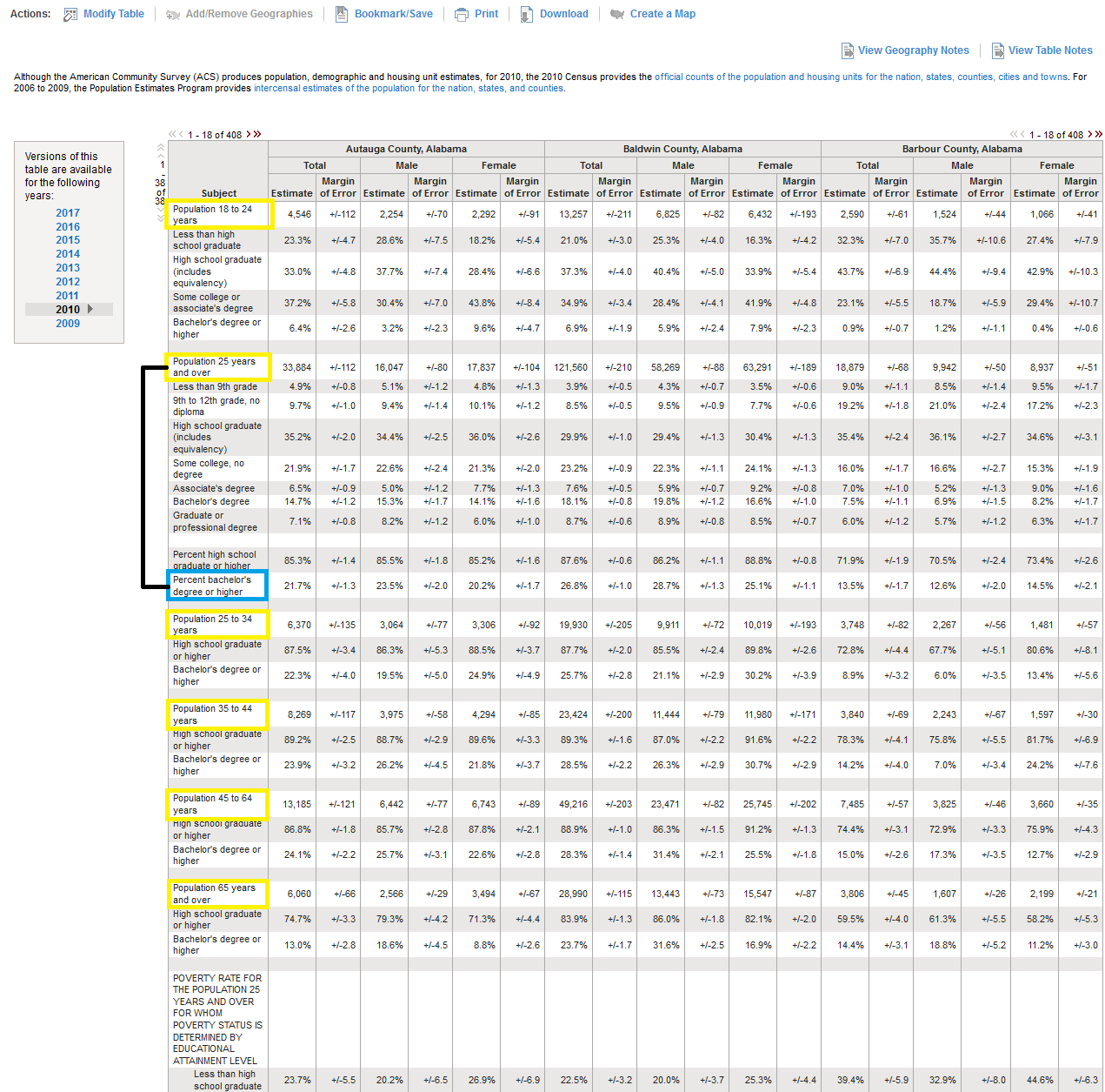
To start answering these questions, you’ll want to go back to the raw, original data and find a codebook or some other identifying documentation. Personally, I recommend this always be your first course of action when you’re unsure about what is contained in a dataset and how it’s labeled. The image below shows an in-browser preview of the Census education data. The data in the left-most column corresponds to what we see in row one of census_edu. We can see that the data is broken down across age categories (yellow boxes) starting at Population 18 to 24 years. The next category begins at Population 25 years and over, and beneath that, we see a sub category (blue box), Percent bachelor’s degree or higher. This should have been our target string all along.

Using the string Bachelor’s degree or higher rather than Percent bachelor’s degree or higher was returning information for age categories we aren’t interested in. We want the measurement that contains the most information about the largest amount of the population in our particular case. So, if we test the string Percent bachelor’s degree or higher, as we do in the code below, we’ll see that R only returns a single column. This allows us to be confident we have selected the correct column now!

census_edu %>%
  select(County = which(str_detect(unlist(.[1,]), "Geography") == T), PercentBachelorOrHigher = which(str_detect(unlist(.[1,]), "Total; Estimate; Percent bachelor's degree or higher") == T)) %>%
  head()

Table 2.4: Properly Identified Column via Combination of Manual Inspection and Conditional Selection
County	PercentBachelorOrHigher
Geography	Total; Estimate; Percent bachelor’s degree or higher
Autauga County, Alabama	21.7
Baldwin County, Alabama	26.8
Barbour County, Alabama	13.5
Bibb County, Alabama	10.0
Blount County, Alabama	12.5

The next verb we use is slice(), which allows us to choose to keep or discard rows by name or position. We discard the first row of the data in this case because it contained the column descriptions, which we made obsolete by renaming the columns to better convey their contents. To discard rows within the slice() function, simply precede the desired row number with the subtraction symbol as I do below.

Next, we use mutate(), which allows us to create new columns or convert existing columns into something new. In this case, we convert PercentBachelororHigher, from a factor variable to a numeric variable and multiply it by 0.01 to convert it into a more conventional decimal form representation of percent data.

Finally, some of the data was missing or non-numeric, meaning that R returns NA for some counties when we asked it to perform the mutation. Since we don’t have that data for those counties, we simply drop them from the final data by using the drop_na() function. Table 2.5 shows what our clean data should resemble now. With just a few lines of code, we tidied up our data to a nice workable format! Compare this to the mess we started with that is Table 2.1, and you’ll start to get a feel for how powerful R can be when organizing and tidying up data!

census_edu_clean <- census_edu %>%
  select(County = which(str_detect(unlist(.[1,]), "Geography") == T), PercentBachelorOrHigher = which(str_detect(unlist(.[1,]), "Total; Estimate; Percent bachelor's degree or higher") == T)) %>%
  slice(-1) %>%
  mutate(PercentBachelorOrHigher = as.numeric(levels(PercentBachelorOrHigher))[PercentBachelorOrHigher] * 0.01) %>%
  drop_na()

head(census_edu_clean)

Table 2.5: Cleaned Education Data Preview
County	PercentBachelorOrHigher
Autauga County, Alabama	0.217
Baldwin County, Alabama	0.268
Barbour County, Alabama	0.135
Bibb County, Alabama	0.100
Blount County, Alabama	0.125
Bullock County, Alabama	0.120

Voila! With just a few lines of code, we tidied up our data to a nice workable format! Compare this to the mess we started with that is Table 2.1, and you’ll start to get a feel for how powerful R can be when organizing and tidying up data!

Unfortunately, the process doesn’t stop there, however. We should make sure that we have the expected number of observations left over, and if we don’t, we need to find out why in the event that it might be correctable. To do that, we can use the base R function nrow(). Note that the drop_na() function will drop the entire row wherever there are NA’s in a column. Knowing that, we should compare the number of rows we have left after using drop_na() to the number of rows we had to begin with in census_edu minus one. We compare to census_edu - 1 because we used slice() to intentionally get rid of the first row of data already.

nrow(census_edu) - 1

## [1] 657

nrow(census_edu_clean)

## [1] 657

Perfect! The numbers of rows in each match, so we’re good to go on the education data. Now that we know the basics of how to clean data in R, let’s continue grabbing some more of the other variables we need.

2.5 Downloading the Census Age Data

To obtain the age data, follow the same steps as detailed in Section 2.2, but replace Education -> Educational Attainment from the topics list with Age & Sex -> Age. Download the dataset 2010 SF1 100% Data, and extract it to the same Census Data folder I recommended before. Once downloaded, you can import using similar code to before.

census_age <- as_tibble(read.csv(here("Census Data", "DEC_10_SF1_QTP1_with_ann.csv"), header = T))

head(census_age)

Viewing the data demonstrates the same problems exist for this data as the education data.

Table 2.6: Uncleaned Age Data Preview
GEO.id	GEO.id2	GEO.display.label	SUBHD0101_S01	SUBHD0102_S01	SUBHD0103_S01	SUBHD0201_S01	SUBHD0202_S01	SUBHD0203_S01	HD03_S01	SUBHD0101_S02	SUBHD0102_S02	SUBHD0103_S02	SUBHD0201_S02	SUBHD0202_S02	SUBHD0203_S02	HD03_S02	SUBHD0101_S03	SUBHD0102_S03	SUBHD0103_S03	SUBHD0201_S03	SUBHD0202_S03	SUBHD0203_S03	HD03_S03	SUBHD0101_S04	SUBHD0102_S04	SUBHD0103_S04	SUBHD0201_S04	SUBHD0202_S04	SUBHD0203_S04	HD03_S04	SUBHD0101_S05	SUBHD0102_S05	SUBHD0103_S05	SUBHD0201_S05	SUBHD0202_S05	SUBHD0203_S05	HD03_S05	SUBHD0101_S06	SUBHD0102_S06	SUBHD0103_S06	SUBHD0201_S06	SUBHD0202_S06	SUBHD0203_S06	HD03_S06	SUBHD0101_S07	SUBHD0102_S07	SUBHD0103_S07	SUBHD0201_S07	SUBHD0202_S07	SUBHD0203_S07	HD03_S07	SUBHD0101_S08	SUBHD0102_S08	SUBHD0103_S08	SUBHD0201_S08	SUBHD0202_S08	SUBHD0203_S08	HD03_S08	SUBHD0101_S09	SUBHD0102_S09	SUBHD0103_S09	SUBHD0201_S09	SUBHD0202_S09	SUBHD0203_S09	HD03_S09	SUBHD0101_S10	SUBHD0102_S10	SUBHD0103_S10	SUBHD0201_S10	SUBHD0202_S10	SUBHD0203_S10	HD03_S10	SUBHD0101_S11	SUBHD0102_S11	SUBHD0103_S11	SUBHD0201_S11	SUBHD0202_S11	SUBHD0203_S11	HD03_S11	SUBHD0101_S12	SUBHD0102_S12	SUBHD0103_S12	SUBHD0201_S12	SUBHD0202_S12	SUBHD0203_S12	HD03_S12	SUBHD0101_S13	SUBHD0102_S13	SUBHD0103_S13	SUBHD0201_S13	SUBHD0202_S13	SUBHD0203_S13	HD03_S13	SUBHD0101_S14	SUBHD0102_S14	SUBHD0103_S14	SUBHD0201_S14	SUBHD0202_S14	SUBHD0203_S14	HD03_S14	SUBHD0101_S15	SUBHD0102_S15	SUBHD0103_S15	SUBHD0201_S15	SUBHD0202_S15	SUBHD0203_S15	HD03_S15	SUBHD0101_S16	SUBHD0102_S16	SUBHD0103_S16	SUBHD0201_S16	SUBHD0202_S16	SUBHD0203_S16	HD03_S16	SUBHD0101_S17	SUBHD0102_S17	SUBHD0103_S17	SUBHD0201_S17	SUBHD0202_S17	SUBHD0203_S17	HD03_S17	SUBHD0101_S18	SUBHD0102_S18	SUBHD0103_S18	SUBHD0201_S18	SUBHD0202_S18	SUBHD0203_S18	HD03_S18	SUBHD0101_S19	SUBHD0102_S19	SUBHD0103_S19	SUBHD0201_S19	SUBHD0202_S19	SUBHD0203_S19	HD03_S19	SUBHD0101_S20	SUBHD0102_S20	SUBHD0103_S20	SUBHD0201_S20	SUBHD0202_S20	SUBHD0203_S20	HD03_S20	SUBHD0101_S21	SUBHD0102_S21	SUBHD0103_S21	SUBHD0201_S21	SUBHD0202_S21	SUBHD0203_S21	HD03_S21	SUBHD0101_S22	SUBHD0102_S22	SUBHD0103_S22	SUBHD0201_S22	SUBHD0202_S22	SUBHD0203_S22	HD03_S22	SUBHD0101_S23	SUBHD0102_S23	SUBHD0103_S23	SUBHD0201_S23	SUBHD0202_S23	SUBHD0203_S23	HD03_S23	SUBHD0101_S24	SUBHD0102_S24	SUBHD0103_S24	SUBHD0201_S24	SUBHD0202_S24	SUBHD0203_S24	HD03_S24	SUBHD0101_S25	SUBHD0102_S25	SUBHD0103_S25	SUBHD0201_S25	SUBHD0202_S25	SUBHD0203_S25	HD03_S25	SUBHD0101_S26	SUBHD0102_S26	SUBHD0103_S26	SUBHD0201_S26	SUBHD0202_S26	SUBHD0203_S26	HD03_S26	SUBHD0101_S27	SUBHD0102_S27	SUBHD0103_S27	SUBHD0201_S27	SUBHD0202_S27	SUBHD0203_S27	HD03_S27	SUBHD0101_S28	SUBHD0102_S28	SUBHD0103_S28	SUBHD0201_S28	SUBHD0202_S28	SUBHD0203_S28	HD03_S28	SUBHD0101_S29	SUBHD0102_S29	SUBHD0103_S29	SUBHD0201_S29	SUBHD0202_S29	SUBHD0203_S29	HD03_S29	SUBHD0101_S30	SUBHD0102_S30	SUBHD0103_S30	SUBHD0201_S30	SUBHD0202_S30	SUBHD0203_S30	HD03_S30	SUBHD0101_S31	SUBHD0102_S31	SUBHD0103_S31	SUBHD0201_S31	SUBHD0202_S31	SUBHD0203_S31	HD03_S31	SUBHD0101_S32	SUBHD0102_S32	SUBHD0103_S32	SUBHD0201_S32	SUBHD0202_S32	SUBHD0203_S32	HD03_S32	SUBHD0101_S33	SUBHD0102_S33	SUBHD0103_S33	SUBHD0201_S33	SUBHD0202_S33	SUBHD0203_S33	HD03_S33	SUBHD0101_S34	SUBHD0102_S34	SUBHD0103_S34	SUBHD0201_S34	SUBHD0202_S34	SUBHD0203_S34	HD03_S34	SUBHD0101_S35	SUBHD0102_S35	SUBHD0103_S35	SUBHD0201_S35	SUBHD0202_S35	SUBHD0203_S35	HD03_S35	SUBHD0101_S36	SUBHD0102_S36	SUBHD0103_S36	SUBHD0201_S36	SUBHD0202_S36	SUBHD0203_S36	HD03_S36	SUBHD0101_S37	SUBHD0102_S37	SUBHD0103_S37	SUBHD0201_S37	SUBHD0202_S37	SUBHD0203_S37	HD03_S37	SUBHD0101_S38	SUBHD0102_S38	SUBHD0103_S38	SUBHD0201_S38	SUBHD0202_S38	SUBHD0203_S38	HD03_S38	SUBHD0101_S39	SUBHD0102_S39	SUBHD0103_S39	SUBHD0201_S39	SUBHD0202_S39	SUBHD0203_S39	HD03_S39	SUBHD0101_S40	SUBHD0102_S40	SUBHD0103_S40	SUBHD0201_S40	SUBHD0202_S40	SUBHD0203_S40	HD03_S40	SUBHD0101_S41	SUBHD0102_S41	SUBHD0103_S41	SUBHD0201_S41	SUBHD0202_S41	SUBHD0203_S41	HD03_S41
Id	Id2	Geography	Number - Both sexes; Total population	Number - Male; Total population	Number - Female; Total population	Percent - Both sexes; Total population	Percent - Male; Total population	Percent - Female; Total population	Males per 100 females; Total population	Number - Both sexes; Total population - Under 5 years	Number - Male; Total population - Under 5 years	Number - Female; Total population - Under 5 years	Percent - Both sexes; Total population - Under 5 years	Percent - Male; Total population - Under 5 years	Percent - Female; Total population - Under 5 years	Males per 100 females; Total population - Under 5 years	Number - Both sexes; Total population - 5 to 9 years	Number - Male; Total population - 5 to 9 years	Number - Female; Total population - 5 to 9 years	Percent - Both sexes; Total population - 5 to 9 years	Percent - Male; Total population - 5 to 9 years	Percent - Female; Total population - 5 to 9 years	Males per 100 females; Total population - 5 to 9 years	Number - Both sexes; Total population - 10 to 14 years	Number - Male; Total population - 10 to 14 years	Number - Female; Total population - 10 to 14 years	Percent - Both sexes; Total population - 10 to 14 years	Percent - Male; Total population - 10 to 14 years	Percent - Female; Total population - 10 to 14 years	Males per 100 females; Total population - 10 to 14 years	Number - Both sexes; Total population - 15 to 19 years	Number - Male; Total population - 15 to 19 years	Number - Female; Total population - 15 to 19 years	Percent - Both sexes; Total population - 15 to 19 years	Percent - Male; Total population - 15 to 19 years	Percent - Female; Total population - 15 to 19 years	Males per 100 females; Total population - 15 to 19 years	Number - Both sexes; Total population - 20 to 24 years	Number - Male; Total population - 20 to 24 years	Number - Female; Total population - 20 to 24 years	Percent - Both sexes; Total population - 20 to 24 years	Percent - Male; Total population - 20 to 24 years	Percent - Female; Total population - 20 to 24 years	Males per 100 females; Total population - 20 to 24 years	Number - Both sexes; Total population - 25 to 29 years	Number - Male; Total population - 25 to 29 years	Number - Female; Total population - 25 to 29 years	Percent - Both sexes; Total population - 25 to 29 years	Percent - Male; Total population - 25 to 29 years	Percent - Female; Total population - 25 to 29 years	Males per 100 females; Total population - 25 to 29 years	Number - Both sexes; Total population - 30 to 34 years	Number - Male; Total population - 30 to 34 years	Number - Female; Total population - 30 to 34 years	Percent - Both sexes; Total population - 30 to 34 years	Percent - Male; Total population - 30 to 34 years	Percent - Female; Total population - 30 to 34 years	Males per 100 females; Total population - 30 to 34 years	Number - Both sexes; Total population - 35 to 39 years	Number - Male; Total population - 35 to 39 years	Number - Female; Total population - 35 to 39 years	Percent - Both sexes; Total population - 35 to 39 years	Percent - Male; Total population - 35 to 39 years	Percent - Female; Total population - 35 to 39 years	Males per 100 females; Total population - 35 to 39 years	Number - Both sexes; Total population - 40 to 44 years	Number - Male; Total population - 40 to 44 years	Number - Female; Total population - 40 to 44 years	Percent - Both sexes; Total population - 40 to 44 years	Percent - Male; Total population - 40 to 44 years	Percent - Female; Total population - 40 to 44 years	Males per 100 females; Total population - 40 to 44 years	Number - Both sexes; Total population - 45 to 49 years	Number - Male; Total population - 45 to 49 years	Number - Female; Total population - 45 to 49 years	Percent - Both sexes; Total population - 45 to 49 years	Percent - Male; Total population - 45 to 49 years	Percent - Female; Total population - 45 to 49 years	Males per 100 females; Total population - 45 to 49 years	Number - Both sexes; Total population - 50 to 54 years	Number - Male; Total population - 50 to 54 years	Number - Female; Total population - 50 to 54 years	Percent - Both sexes; Total population - 50 to 54 years	Percent - Male; Total population - 50 to 54 years	Percent - Female; Total population - 50 to 54 years	Males per 100 females; Total population - 50 to 54 years	Number - Both sexes; Total population - 55 to 59 years	Number - Male; Total population - 55 to 59 years	Number - Female; Total population - 55 to 59 years	Percent - Both sexes; Total population - 55 to 59 years	Percent - Male; Total population - 55 to 59 years	Percent - Female; Total population - 55 to 59 years	Males per 100 females; Total population - 55 to 59 years	Number - Both sexes; Total population - 60 to 64 years	Number - Male; Total population - 60 to 64 years	Number - Female; Total population - 60 to 64 years	Percent - Both sexes; Total population - 60 to 64 years	Percent - Male; Total population - 60 to 64 years	Percent - Female; Total population - 60 to 64 years	Males per 100 females; Total population - 60 to 64 years	Number - Both sexes; Total population - 65 to 69 years	Number - Male; Total population - 65 to 69 years	Number - Female; Total population - 65 to 69 years	Percent - Both sexes; Total population - 65 to 69 years	Percent - Male; Total population - 65 to 69 years	Percent - Female; Total population - 65 to 69 years	Males per 100 females; Total population - 65 to 69 years	Number - Both sexes; Total population - 70 to 74 years	Number - Male; Total population - 70 to 74 years	Number - Female; Total population - 70 to 74 years	Percent - Both sexes; Total population - 70 to 74 years	Percent - Male; Total population - 70 to 74 years	Percent - Female; Total population - 70 to 74 years	Males per 100 females; Total population - 70 to 74 years	Number - Both sexes; Total population - 75 to 79 years	Number - Male; Total population - 75 to 79 years	Number - Female; Total population - 75 to 79 years	Percent - Both sexes; Total population - 75 to 79 years	Percent - Male; Total population - 75 to 79 years	Percent - Female; Total population - 75 to 79 years	Males per 100 females; Total population - 75 to 79 years	Number - Both sexes; Total population - 80 to 84 years	Number - Male; Total population - 80 to 84 years	Number - Female; Total population - 80 to 84 years	Percent - Both sexes; Total population - 80 to 84 years	Percent - Male; Total population - 80 to 84 years	Percent - Female; Total population - 80 to 84 years	Males per 100 females; Total population - 80 to 84 years	Number - Both sexes; Total population - 85 to 89 years	Number - Male; Total population - 85 to 89 years	Number - Female; Total population - 85 to 89 years	Percent - Both sexes; Total population - 85 to 89 years	Percent - Male; Total population - 85 to 89 years	Percent - Female; Total population - 85 to 89 years	Males per 100 females; Total population - 85 to 89 years	Number - Both sexes; Total population - 90 years and over	Number - Male; Total population - 90 years and over	Number - Female; Total population - 90 years and over	Percent - Both sexes; Total population - 90 years and over	Percent - Male; Total population - 90 years and over	Percent - Female; Total population - 90 years and over	Males per 100 females; Total population - 90 years and over	Number - Both sexes; Total population - Under 18 years	Number - Male; Total population - Under 18 years	Number - Female; Total population - Under 18 years	Percent - Both sexes; Total population - Under 18 years	Percent - Male; Total population - Under 18 years	Percent - Female; Total population - Under 18 years	Males per 100 females; Total population - Under 18 years	Number - Both sexes; Total population - 18 to 64 years	Number - Male; Total population - 18 to 64 years	Number - Female; Total population - 18 to 64 years	Percent - Both sexes; Total population - 18 to 64 years	Percent - Male; Total population - 18 to 64 years	Percent - Female; Total population - 18 to 64 years	Males per 100 females; Total population - 18 to 64 years	Number - Both sexes; Total population - 18 to 64 years - 18 to 24 years	Number - Male; Total population - 18 to 64 years - 18 to 24 years	Number - Female; Total population - 18 to 64 years - 18 to 24 years	Percent - Both sexes; Total population - 18 to 64 years - 18 to 24 years	Percent - Male; Total population - 18 to 64 years - 18 to 24 years	Percent - Female; Total population - 18 to 64 years - 18 to 24 years	Males per 100 females; Total population - 18 to 64 years - 18 to 24 years	Number - Both sexes; Total population - 18 to 64 years - 25 to 44 years	Number - Male; Total population - 18 to 64 years - 25 to 44 years	Number - Female; Total population - 18 to 64 years - 25 to 44 years	Percent - Both sexes; Total population - 18 to 64 years - 25 to 44 years	Percent - Male; Total population - 18 to 64 years - 25 to 44 years	Percent - Female; Total population - 18 to 64 years - 25 to 44 years	Males per 100 females; Total population - 18 to 64 years - 25 to 44 years	Number - Both sexes; Total population - 18 to 64 years - 25 to 44 years - 25 to 34 years	Number - Male; Total population - 18 to 64 years - 25 to 44 years - 25 to 34 years	Number - Female; Total population - 18 to 64 years - 25 to 44 years - 25 to 34 years	Percent - Both sexes; Total population - 18 to 64 years - 25 to 44 years - 25 to 34 years	Percent - Male; Total population - 18 to 64 years - 25 to 44 years - 25 to 34 years	Percent - Female; Total population - 18 to 64 years - 25 to 44 years - 25 to 34 years	Males per 100 females; Total population - 18 to 64 years - 25 to 44 years - 25 to 34 years	Number - Both sexes; Total population - 18 to 64 years - 25 to 44 years - 35 to 44 years	Number - Male; Total population - 18 to 64 years - 25 to 44 years - 35 to 44 years	Number - Female; Total population - 18 to 64 years - 25 to 44 years - 35 to 44 years	Percent - Both sexes; Total population - 18 to 64 years - 25 to 44 years - 35 to 44 years	Percent - Male; Total population - 18 to 64 years - 25 to 44 years - 35 to 44 years	Percent - Female; Total population - 18 to 64 years - 25 to 44 years - 35 to 44 years	Males per 100 females; Total population - 18 to 64 years - 25 to 44 years - 35 to 44 years	Number - Both sexes; Total population - 18 to 64 years - 45 to 64 years	Number - Male; Total population - 18 to 64 years - 45 to 64 years	Number - Female; Total population - 18 to 64 years - 45 to 64 years	Percent - Both sexes; Total population - 18 to 64 years - 45 to 64 years	Percent - Male; Total population - 18 to 64 years - 45 to 64 years	Percent - Female; Total population - 18 to 64 years - 45 to 64 years	Males per 100 females; Total population - 18 to 64 years - 45 to 64 years	Number - Both sexes; Total population - 18 to 64 years - 45 to 64 years - 45 to 54 years	Number - Male; Total population - 18 to 64 years - 45 to 64 years - 45 to 54 years	Number - Female; Total population - 18 to 64 years - 45 to 64 years - 45 to 54 years	Percent - Both sexes; Total population - 18 to 64 years - 45 to 64 years - 45 to 54 years	Percent - Male; Total population - 18 to 64 years - 45 to 64 years - 45 to 54 years	Percent - Female; Total population - 18 to 64 years - 45 to 64 years - 45 to 54 years	Males per 100 females; Total population - 18 to 64 years - 45 to 64 years - 45 to 54 years	Number - Both sexes; Total population - 18 to 64 years - 45 to 64 years - 55 to 64 years	Number - Male; Total population - 18 to 64 years - 45 to 64 years - 55 to 64 years	Number - Female; Total population - 18 to 64 years - 45 to 64 years - 55 to 64 years	Percent - Both sexes; Total population - 18 to 64 years - 45 to 64 years - 55 to 64 years	Percent - Male; Total population - 18 to 64 years - 45 to 64 years - 55 to 64 years	Percent - Female; Total population - 18 to 64 years - 45 to 64 years - 55 to 64 years	Males per 100 females; Total population - 18 to 64 years - 45 to 64 years - 55 to 64 years	Number - Both sexes; Total population - 65 years and over	Number - Male; Total population - 65 years and over	Number - Female; Total population - 65 years and over	Percent - Both sexes; Total population - 65 years and over	Percent - Male; Total population - 65 years and over	Percent - Female; Total population - 65 years and over	Males per 100 females; Total population - 65 years and over	Number - Both sexes; Total population - 65 years and over - 65 to 74 years	Number - Male; Total population - 65 years and over - 65 to 74 years	Number - Female; Total population - 65 years and over - 65 to 74 years	Percent - Both sexes; Total population - 65 years and over - 65 to 74 years	Percent - Male; Total population - 65 years and over - 65 to 74 years	Percent - Female; Total population - 65 years and over - 65 to 74 years	Males per 100 females; Total population - 65 years and over - 65 to 74 years	Number - Both sexes; Total population - 65 years and over - 75 to 84 years	Number - Male; Total population - 65 years and over - 75 to 84 years	Number - Female; Total population - 65 years and over - 75 to 84 years	Percent - Both sexes; Total population - 65 years and over - 75 to 84 years	Percent - Male; Total population - 65 years and over - 75 to 84 years	Percent - Female; Total population - 65 years and over - 75 to 84 years	Males per 100 females; Total population - 65 years and over - 75 to 84 years	Number - Both sexes; Total population - 65 years and over - 85 years and over	Number - Male; Total population - 65 years and over - 85 years and over	Number - Female; Total population - 65 years and over - 85 years and over	Percent - Both sexes; Total population - 65 years and over - 85 years and over	Percent - Male; Total population - 65 years and over - 85 years and over	Percent - Female; Total population - 65 years and over - 85 years and over	Males per 100 females; Total population - 65 years and over - 85 years and over	Number - Both sexes; Total population - 16 years and over	Number - Male; Total population - 16 years and over	Number - Female; Total population - 16 years and over	Percent - Both sexes; Total population - 16 years and over	Percent - Male; Total population - 16 years and over	Percent - Female; Total population - 16 years and over	Males per 100 females; Total population - 16 years and over	Number - Both sexes; Total population - 18 years and over	Number - Male; Total population - 18 years and over	Number - Female; Total population - 18 years and over	Percent - Both sexes; Total population - 18 years and over	Percent - Male; Total population - 18 years and over	Percent - Female; Total population - 18 years and over	Males per 100 females; Total population - 18 years and over	Number - Both sexes; Total population - 21 years and over	Number - Male; Total population - 21 years and over	Number - Female; Total population - 21 years and over	Percent - Both sexes; Total population - 21 years and over	Percent - Male; Total population - 21 years and over	Percent - Female; Total population - 21 years and over	Males per 100 females; Total population - 21 years and over	Number - Both sexes; Total population - 60 years and over	Number - Male; Total population - 60 years and over	Number - Female; Total population - 60 years and over	Percent - Both sexes; Total population - 60 years and over	Percent - Male; Total population - 60 years and over	Percent - Female; Total population - 60 years and over	Males per 100 females; Total population - 60 years and over	Number - Both sexes; Total population - 62 years and over	Number - Male; Total population - 62 years and over	Number - Female; Total population - 62 years and over	Percent - Both sexes; Total population - 62 years and over	Percent - Male; Total population - 62 years and over	Percent - Female; Total population - 62 years and over	Males per 100 females; Total population - 62 years and over	Number - Both sexes; Total population - 67 years and over	Number - Male; Total population - 67 years and over	Number - Female; Total population - 67 years and over	Percent - Both sexes; Total population - 67 years and over	Percent - Male; Total population - 67 years and over	Percent - Female; Total population - 67 years and over	Males per 100 females; Total population - 67 years and over	Number - Both sexes; Total population - 75 years and over	Number - Male; Total population - 75 years and over	Number - Female; Total population - 75 years and over	Percent - Both sexes; Total population - 75 years and over	Percent - Male; Total population - 75 years and over	Percent - Female; Total population - 75 years and over	Males per 100 females; Total population - 75 years and over	Number - Both sexes; Total population - Median age (years)	Number - Male; Total population - Median age (years)	Number - Female; Total population - Median age (years)	Percent - Both sexes; Total population - Median age (years)	Percent - Male; Total population - Median age (years)	Percent - Female; Total population - Median age (years)	Males per 100 females; Total population - Median age (years)
0500000US01001	01001	Autauga County, Alabama	54571	26569	28002	100.0	100.0	100.0	94.9	3579	1866	1713	6.6	7.0	6.1	108.9	3991	2001	1990	7.3	7.5	7.1	100.6	4290	2171	2119	7.9	8.2	7.6	102.5	4290	2213	2077	7.9	8.3	7.4	106.5	3080	1539	1541	5.6	5.8	5.5	99.9	3157	1543	1614	5.8	5.8	5.8	95.6	3330	1594	1736	6.1	6.0	6.2	91.8	4157	2004	2153	7.6	7.5	7.7	93.1	4086	1974	2112	7.5	7.4	7.5	93.5	4332	2174	2158	7.9	8.2	7.7	100.7	3873	1866	2007	7.1	7.0	7.2	93.0	3083	1524	1559	5.6	5.7	5.6	97.8	2777	1279	1498	5.1	4.8	5.3	85.4	2277	1014	1263	4.2	3.8	4.5	80.3	1736	807	929	3.2	3.0	3.3	86.9	1251	546	705	2.3	2.1	2.5	77.4	731	295	436	1.3	1.1	1.6	67.7	367	113	254	0.7	0.4	0.9	44.5	184	46	138	0.3	0.2	0.5	33.3	14613	7455	7158	26.8	28.1	25.6	104.1	33412	16293	17119	61.2	61.3	61.1	95.2	4617	2335	2282	8.5	8.8	8.1	102.3	14730	7115	7615	27.0	26.8	27.2	93.4	6487	3137	3350	11.9	11.8	12.0	93.6	8243	3978	4265	15.1	15.0	15.2	93.3	14065	6843	7222	25.8	25.8	25.8	94.8	8205	4040	4165	15.0	15.2	14.9	97.0	5860	2803	3057	10.7	10.5	10.9	91.7	6546	2821	3725	12.0	10.6	13.3	75.7	4013	1821	2192	7.4	6.9	7.8	83.1	1982	841	1141	3.6	3.2	4.1	73.7	551	159	392	1.0	0.6	1.4	40.6	41804	20046	21758	76.6	75.4	77.7	92.1	39958	19114	20844	73.2	71.9	74.4	91.7	37756	17968	19788	69.2	67.6	70.7	90.8	9323	4100	5223	17.1	15.4	18.7	78.5	8222	3606	4616	15.1	13.6	16.5	78.1	5614	2403	3211	10.3	9.0	11.5	74.8	2533	1000	1533	4.6	3.8	5.5	65.2	37.0	35.9	37.9	( X )	( X )	( X )	( X )
0500000US01003	01003	Baldwin County, Alabama	182265	89196	93069	100.0	100.0	100.0	95.8	11158	5614	5544	6.1	6.3	6.0	101.3	11599	5832	5767	6.4	6.5	6.2	101.1	11926	6076	5850	6.5	6.8	6.3	103.9	11600	5930	5670	6.4	6.6	6.1	104.6	9449	4793	4656	5.2	5.4	5.0	102.9	10247	5183	5064	5.6	5.8	5.4	102.3	10709	5317	5392	5.9	6.0	5.8	98.6	11558	5725	5833	6.3	6.4	6.3	98.1	11995	5895	6100	6.6	6.6	6.6	96.6	13431	6622	6809	7.4	7.4	7.3	97.3	13490	6425	7065	7.4	7.2	7.6	90.9	12523	5943	6580	6.9	6.7	7.1	90.3	12012	5728	6284	6.6	6.4	6.8	91.2	10174	4895	5279	5.6	5.5	5.7	92.7	7629	3663	3966	4.2	4.1	4.3	92.4	5598	2644	2954	3.1	3.0	3.2	89.5	3934	1735	2199	2.2	1.9	2.4	78.9	2221	863	1358	1.2	1.0	1.5	63.5	1012	313	699	0.6	0.4	0.8	44.8	41898	21226	20672	23.0	23.8	22.2	102.7	109799	53857	55942	60.2	60.4	60.1	96.3	13834	7019	6815	7.6	7.9	7.3	103.0	44509	22120	22389	24.4	24.8	24.1	98.8	20956	10500	10456	11.5	11.8	11.2	100.4	23553	11620	11933	12.9	13.0	12.8	97.4	51456	24718	26738	28.2	27.7	28.7	92.4	26921	13047	13874	14.8	14.6	14.9	94.0	24535	11671	12864	13.5	13.1	13.8	90.7	30568	14113	16455	16.8	15.8	17.7	85.8	17803	8558	9245	9.8	9.6	9.9	92.6	9532	4379	5153	5.2	4.9	5.5	85.0	3233	1176	2057	1.8	1.3	2.2	57.2	145215	70491	74724	79.7	79.0	80.3	94.3	140367	67970	72397	77.0	76.2	77.8	93.9	134024	64731	69293	73.5	72.6	74.5	93.4	42580	19841	22739	23.4	22.2	24.4	87.3	37780	17540	20240	20.7	19.7	21.7	86.7	26301	12059	14242	14.4	13.5	15.3	84.7	12765	5555	7210	7.0	6.2	7.7	77.0	41.1	40.1	42.2	( X )	( X )	( X )	( X )
0500000US01005	01005	Barbour County, Alabama	27457	14576	12881	100.0	100.0	100.0	113.2	1702	847	855	6.2	5.8	6.6	99.1	1642	826	816	6.0	5.7	6.3	101.2	1599	820	779	5.8	5.6	6.0	105.3	1731	919	812	6.3	6.3	6.3	113.2	1794	1048	746	6.5	7.2	5.8	140.5	2010	1212	798	7.3	8.3	6.2	151.9	1808	1162	646	6.6	8.0	5.0	179.9	1819	1046	773	6.6	7.2	6.0	135.3	1809	1069	740	6.6	7.3	5.7	144.5	2108	1164	944	7.7	8.0	7.3	123.3	1910	1000	910	7.0	6.9	7.1	109.9	1817	910	907	6.6	6.2	7.0	100.3	1799	859	940	6.6	5.9	7.3	91.4	1290	631	659	4.7	4.3	5.1	95.8	948	436	512	3.5	3.0	4.0	85.2	685	303	382	2.5	2.1	3.0	79.3	543	195	348	2.0	1.3	2.7	56.0	311	97	214	1.1	0.7	1.7	45.3	132	32	100	0.5	0.2	0.8	32.0	6015	3052	2963	21.9	20.9	23.0	103.0	17533	9830	7703	63.9	67.4	59.8	127.6	2453	1408	1045	8.9	9.7	8.1	134.7	7446	4489	2957	27.1	30.8	23.0	151.8	3818	2374	1444	13.9	16.3	11.2	164.4	3628	2115	1513	13.2	14.5	11.7	139.8	7634	3933	3701	27.8	27.0	28.7	106.3	4018	2164	1854	14.6	14.8	14.4	116.7	3616	1769	1847	13.2	12.1	14.3	95.8	3909	1694	2215	14.2	11.6	17.2	76.5	2238	1067	1171	8.2	7.3	9.1	91.1	1228	498	730	4.5	3.4	5.7	68.2	443	129	314	1.6	0.9	2.4	41.1	22185	11904	10281	80.8	81.7	79.8	115.8	21442	11524	9918	78.1	79.1	77.0	116.2	20435	10974	9461	74.4	75.3	73.4	116.0	5708	2553	3155	20.8	17.5	24.5	80.9	4958	2195	2763	18.1	15.1	21.5	79.4	3353	1414	1939	12.2	9.7	15.1	72.9	1671	627	1044	6.1	4.3	8.1	60.1	39.0	37.2	41.6	( X )	( X )	( X )	( X )
0500000US01007	01007	Bibb County, Alabama	22915	12301	10614	100.0	100.0	100.0	115.9	1378	712	666	6.0	5.8	6.3	106.9	1405	759	646	6.1	6.2	6.1	117.5	1440	771	669	6.3	6.3	6.3	115.2	1543	806	737	6.7	6.6	6.9	109.4	1491	811	680	6.5	6.6	6.4	119.3	1603	987	616	7.0	8.0	5.8	160.2	1646	1013	633	7.2	8.2	6.0	160.0	1747	1003	744	7.6	8.2	7.0	134.8	1635	892	743	7.1	7.3	7.0	120.1	1805	1036	769	7.9	8.4	7.2	134.7	1581	847	734	6.9	6.9	6.9	115.4	1401	734	667	6.1	6.0	6.3	110.0	1334	684	650	5.8	5.6	6.1	105.2	966	456	510	4.2	3.7	4.8	89.4	757	347	410	3.3	2.8	3.9	84.6	549	232	317	2.4	1.9	3.0	73.2	355	138	217	1.5	1.1	2.0	63.6	190	54	136	0.8	0.4	1.3	39.7	89	19	70	0.4	0.2	0.7	27.1	5201	2755	2446	22.7	22.4	23.0	112.6	14808	8300	6508	64.6	67.5	61.3	127.5	2056	1104	952	9.0	9.0	9.0	116.0	6631	3895	2736	28.9	31.7	25.8	142.4	3249	2000	1249	14.2	16.3	11.8	160.1	3382	1895	1487	14.8	15.4	14.0	127.4	6121	3301	2820	26.7	26.8	26.6	117.1	3386	1883	1503	14.8	15.3	14.2	125.3	2735	1418	1317	11.9	11.5	12.4	107.7	2906	1246	1660	12.7	10.1	15.6	75.1	1723	803	920	7.5	6.5	8.7	87.3	904	370	534	3.9	3.0	5.0	69.3	279	73	206	1.2	0.6	1.9	35.4	18372	9900	8472	80.2	80.5	79.8	116.9	17714	9546	8168	77.3	77.6	77.0	116.9	16889	9131	7758	73.7	74.2	73.1	117.7	4240	1930	2310	18.5	15.7	21.8	83.5	3690	1636	2054	16.1	13.3	19.4	79.6	2496	1058	1438	10.9	8.6	13.5	73.6	1183	443	740	5.2	3.6	7.0	59.9	37.8	36.5	39.5	( X )	( X )	( X )	( X )
0500000US01009	01009	Blount County, Alabama	57322	28362	28960	100.0	100.0	100.0	97.9	3616	1805	1811	6.3	6.4	6.3	99.7	3880	1936	1944	6.8	6.8	6.7	99.6	4084	2113	1971	7.1	7.5	6.8	107.2	4033	2139	1894	7.0	7.5	6.5	112.9	3107	1577	1530	5.4	5.6	5.3	103.1	3436	1735	1701	6.0	6.1	5.9	102.0	3441	1730	1711	6.0	6.1	5.9	101.1	3892	1989	1903	6.8	7.0	6.6	104.5	4033	2033	2000	7.0	7.2	6.9	101.7	4163	2096	2067	7.3	7.4	7.1	101.4	3922	1972	1950	6.8	7.0	6.7	101.1	3694	1810	1884	6.4	6.4	6.5	96.1	3582	1700	1882	6.2	6.0	6.5	90.3	2892	1352	1540	5.0	4.8	5.3	87.8	2187	1039	1148	3.8	3.7	4.0	90.5	1517	684	833	2.6	2.4	2.9	82.1	1035	418	617	1.8	1.5	2.1	67.7	541	161	380	0.9	0.6	1.3	42.4	267	73	194	0.5	0.3	0.7	37.6	14106	7194	6912	24.6	25.4	23.9	104.1	34777	17441	17336	60.7	61.5	59.9	100.6	4614	2376	2238	8.0	8.4	7.7	106.2	14802	7487	7315	25.8	26.4	25.3	102.4	6877	3465	3412	12.0	12.2	11.8	101.6	7925	4022	3903	13.8	14.2	13.5	103.0	15361	7578	7783	26.8	26.7	26.9	97.4	8085	4068	4017	14.1	14.3	13.9	101.3	7276	3510	3766	12.7	12.4	13.0	93.2	8439	3727	4712	14.7	13.1	16.3	79.1	5079	2391	2688	8.9	8.4	9.3	89.0	2552	1102	1450	4.5	3.9	5.0	76.0	808	234	574	1.4	0.8	2.0	40.8	44902	22059	22843	78.3	77.8	78.9	96.6	43216	21168	22048	75.4	74.6	76.1	96.0	41054	20029	21025	71.6	70.6	72.6	95.3	12021	5427	6594	21.0	19.1	22.8	82.3	10549	4711	5838	18.4	16.6	20.2	80.7	7239	3181	4058	12.6	11.2	14.0	78.4	3360	1336	2024	5.9	4.7	7.0	66.0	39.0	38.0	40.0	( X )	( X )	( X )	( X )

Fortunately for us, this means we can use nearly identical code to Section 2.4.2 to get the data we want!

2.6 Cleaning the Census Age Data

Cleaning the age data is as simple as changing up the object names to reflect the right data to operate on. I won’t explain what all of the functions we’re using here do again, but if you need a refresher, see Section 2.4. Recalling the contents of the MS dataset (or simply asking R to remind you with names(MS_Model_Dataset_Reduced_Form)), we know that the only age data we need is the percentage of the population under 18 years, i.e. PercentUnder18. For that reason, we’ll use str_detect() to narrow the columns down to those containing the string “Under 18 years” in the first row. Then, by manually inspecting the manageable output of the first selection, we can write the next selection. The output of the first two lines returns the following.

census_age_clean <- census_age %>%
  select(which(str_detect(unlist(.[1,]), "Geography") == T), which(str_detect(unlist(.[1,]), "Under 18 years") == T))

head(census_age_clean)

Table 2.7: Preview of First Age Data Selection
GEO.display.label	SUBHD0101_S21	SUBHD0102_S21	SUBHD0103_S21	SUBHD0201_S21	SUBHD0202_S21	SUBHD0203_S21	HD03_S21
Geography	Number - Both sexes; Total population - Under 18 years	Number - Male; Total population - Under 18 years	Number - Female; Total population - Under 18 years	Percent - Both sexes; Total population - Under 18 years	Percent - Male; Total population - Under 18 years	Percent - Female; Total population - Under 18 years	Males per 100 females; Total population - Under 18 years
Autauga County, Alabama	14613	7455	7158	26.8	28.1	25.6	104.1
Baldwin County, Alabama	41898	21226	20672	23.0	23.8	22.2	102.7
Barbour County, Alabama	6015	3052	2963	21.9	20.9	23.0	103.0
Bibb County, Alabama	5201	2755	2446	22.7	22.4	23.0	112.6
Blount County, Alabama	14106	7194	6912	24.6	25.4	23.9	104.1

Looking at this subset of the data and scrolling right to inspect the descriptions provided in the first row of each column, you will see that column 5 contains the description “Percent - Both sexes; Total population - Under 18 years”. This matches the data that we need, which is why in the second select() function we specify column 5 to be kept and rename it PercentUnder18, i.e. select(County = 1, PercentUnder18 = 5). The rest of the operations are identical to those used in Section 2.4.

census_age_clean <- census_age %>%
  select(which(str_detect(unlist(.[1,]), "Geography") == T), which(str_detect(unlist(.[1,]), "Under 18 years") == T)) %>%
  select(County = 1, PercentUnder18 = 5) %>%
  slice(-1) %>%
  mutate(PercentUnder18 = as.numeric(levels(PercentUnder18))[PercentUnder18] * 0.01) %>% 
  drop_na()

head(census_age)

Table 2.8: Cleaned Age Data Preview
County	PercentUnder18
Autauga County, Alabama	0.268
Baldwin County, Alabama	0.230
Barbour County, Alabama	0.219
Bibb County, Alabama	0.227
Blount County, Alabama	0.246
Bullock County, Alabama	0.223

Once again, we need to do our due diligence to make sure we didn’t lose any observations that could have been salvaged by checking the number of rows in census_age_clean after dropping NA’s and comparing it to the number of rows in census_age minus one.

nrow(census_age) - 1

## [1] 657

nrow(census_age_clean)

## [1] 657

Seeing no difference, we can stop here and move on to the population data.

2.7 Downloading the Census Population Data

To obtain the population data, follow the steps from Section 2.2 again, but replace Education -> Educational Attainment from the topics list with Basic Count/Estimate -> Population Total. Download the dataset 2010 Demographic Profile SF, and again extract it to the same Census Data folder I recommended before. Once downloaded, you can, again, import using similar code to before. Note that, while the 2010 total population is not included in the Mississippi data, we will need it to generate some of the measures we intend to create later, and that’s why we go ahead and grab it now.

census_totalpop2010 <- read.csv(here("Census Data", "DEC_10_SF1_QTP1_with_ann.csv"), header = T) %>%
  as_tibble()

head(census_totalpop2010)

Viewing the data demonstrates the same problems exist for this data as the education and age data.

Table 2.9: Uncleaned Population Data Preview
GEO.id	GEO.id2	GEO.display.label	SUBHD0101_S01	SUBHD0102_S01	SUBHD0103_S01	SUBHD0201_S01	SUBHD0202_S01	SUBHD0203_S01	HD03_S01	SUBHD0101_S02	SUBHD0102_S02	SUBHD0103_S02	SUBHD0201_S02	SUBHD0202_S02	SUBHD0203_S02	HD03_S02	SUBHD0101_S03	SUBHD0102_S03	SUBHD0103_S03	SUBHD0201_S03	SUBHD0202_S03	SUBHD0203_S03	HD03_S03	SUBHD0101_S04	SUBHD0102_S04	SUBHD0103_S04	SUBHD0201_S04	SUBHD0202_S04	SUBHD0203_S04	HD03_S04	SUBHD0101_S05	SUBHD0102_S05	SUBHD0103_S05	SUBHD0201_S05	SUBHD0202_S05	SUBHD0203_S05	HD03_S05	SUBHD0101_S06	SUBHD0102_S06	SUBHD0103_S06	SUBHD0201_S06	SUBHD0202_S06	SUBHD0203_S06	HD03_S06	SUBHD0101_S07	SUBHD0102_S07	SUBHD0103_S07	SUBHD0201_S07	SUBHD0202_S07	SUBHD0203_S07	HD03_S07	SUBHD0101_S08	SUBHD0102_S08	SUBHD0103_S08	SUBHD0201_S08	SUBHD0202_S08	SUBHD0203_S08	HD03_S08	SUBHD0101_S09	SUBHD0102_S09	SUBHD0103_S09	SUBHD0201_S09	SUBHD0202_S09	SUBHD0203_S09	HD03_S09	SUBHD0101_S10	SUBHD0102_S10	SUBHD0103_S10	SUBHD0201_S10	SUBHD0202_S10	SUBHD0203_S10	HD03_S10	SUBHD0101_S11	SUBHD0102_S11	SUBHD0103_S11	SUBHD0201_S11	SUBHD0202_S11	SUBHD0203_S11	HD03_S11	SUBHD0101_S12	SUBHD0102_S12	SUBHD0103_S12	SUBHD0201_S12	SUBHD0202_S12	SUBHD0203_S12	HD03_S12	SUBHD0101_S13	SUBHD0102_S13	SUBHD0103_S13	SUBHD0201_S13	SUBHD0202_S13	SUBHD0203_S13	HD03_S13	SUBHD0101_S14	SUBHD0102_S14	SUBHD0103_S14	SUBHD0201_S14	SUBHD0202_S14	SUBHD0203_S14	HD03_S14	SUBHD0101_S15	SUBHD0102_S15	SUBHD0103_S15	SUBHD0201_S15	SUBHD0202_S15	SUBHD0203_S15	HD03_S15	SUBHD0101_S16	SUBHD0102_S16	SUBHD0103_S16	SUBHD0201_S16	SUBHD0202_S16	SUBHD0203_S16	HD03_S16	SUBHD0101_S17	SUBHD0102_S17	SUBHD0103_S17	SUBHD0201_S17	SUBHD0202_S17	SUBHD0203_S17	HD03_S17	SUBHD0101_S18	SUBHD0102_S18	SUBHD0103_S18	SUBHD0201_S18	SUBHD0202_S18	SUBHD0203_S18	HD03_S18	SUBHD0101_S19	SUBHD0102_S19	SUBHD0103_S19	SUBHD0201_S19	SUBHD0202_S19	SUBHD0203_S19	HD03_S19	SUBHD0101_S20	SUBHD0102_S20	SUBHD0103_S20	SUBHD0201_S20	SUBHD0202_S20	SUBHD0203_S20	HD03_S20	SUBHD0101_S21	SUBHD0102_S21	SUBHD0103_S21	SUBHD0201_S21	SUBHD0202_S21	SUBHD0203_S21	HD03_S21	SUBHD0101_S22	SUBHD0102_S22	SUBHD0103_S22	SUBHD0201_S22	SUBHD0202_S22	SUBHD0203_S22	HD03_S22	SUBHD0101_S23	SUBHD0102_S23	SUBHD0103_S23	SUBHD0201_S23	SUBHD0202_S23	SUBHD0203_S23	HD03_S23	SUBHD0101_S24	SUBHD0102_S24	SUBHD0103_S24	SUBHD0201_S24	SUBHD0202_S24	SUBHD0203_S24	HD03_S24	SUBHD0101_S25	SUBHD0102_S25	SUBHD0103_S25	SUBHD0201_S25	SUBHD0202_S25	SUBHD0203_S25	HD03_S25	SUBHD0101_S26	SUBHD0102_S26	SUBHD0103_S26	SUBHD0201_S26	SUBHD0202_S26	SUBHD0203_S26	HD03_S26	SUBHD0101_S27	SUBHD0102_S27	SUBHD0103_S27	SUBHD0201_S27	SUBHD0202_S27	SUBHD0203_S27	HD03_S27	SUBHD0101_S28	SUBHD0102_S28	SUBHD0103_S28	SUBHD0201_S28	SUBHD0202_S28	SUBHD0203_S28	HD03_S28	SUBHD0101_S29	SUBHD0102_S29	SUBHD0103_S29	SUBHD0201_S29	SUBHD0202_S29	SUBHD0203_S29	HD03_S29	SUBHD0101_S30	SUBHD0102_S30	SUBHD0103_S30	SUBHD0201_S30	SUBHD0202_S30	SUBHD0203_S30	HD03_S30	SUBHD0101_S31	SUBHD0102_S31	SUBHD0103_S31	SUBHD0201_S31	SUBHD0202_S31	SUBHD0203_S31	HD03_S31	SUBHD0101_S32	SUBHD0102_S32	SUBHD0103_S32	SUBHD0201_S32	SUBHD0202_S32	SUBHD0203_S32	HD03_S32	SUBHD0101_S33	SUBHD0102_S33	SUBHD0103_S33	SUBHD0201_S33	SUBHD0202_S33	SUBHD0203_S33	HD03_S33	SUBHD0101_S34	SUBHD0102_S34	SUBHD0103_S34	SUBHD0201_S34	SUBHD0202_S34	SUBHD0203_S34	HD03_S34	SUBHD0101_S35	SUBHD0102_S35	SUBHD0103_S35	SUBHD0201_S35	SUBHD0202_S35	SUBHD0203_S35	HD03_S35	SUBHD0101_S36	SUBHD0102_S36	SUBHD0103_S36	SUBHD0201_S36	SUBHD0202_S36	SUBHD0203_S36	HD03_S36	SUBHD0101_S37	SUBHD0102_S37	SUBHD0103_S37	SUBHD0201_S37	SUBHD0202_S37	SUBHD0203_S37	HD03_S37	SUBHD0101_S38	SUBHD0102_S38	SUBHD0103_S38	SUBHD0201_S38	SUBHD0202_S38	SUBHD0203_S38	HD03_S38	SUBHD0101_S39	SUBHD0102_S39	SUBHD0103_S39	SUBHD0201_S39	SUBHD0202_S39	SUBHD0203_S39	HD03_S39	SUBHD0101_S40	SUBHD0102_S40	SUBHD0103_S40	SUBHD0201_S40	SUBHD0202_S40	SUBHD0203_S40	HD03_S40	SUBHD0101_S41	SUBHD0102_S41	SUBHD0103_S41	SUBHD0201_S41	SUBHD0202_S41	SUBHD0203_S41	HD03_S41
Id	Id2	Geography	Number - Both sexes; Total population	Number - Male; Total population	Number - Female; Total population	Percent - Both sexes; Total population	Percent - Male; Total population	Percent - Female; Total population	Males per 100 females; Total population	Number - Both sexes; Total population - Under 5 years	Number - Male; Total population - Under 5 years	Number - Female; Total population - Under 5 years	Percent - Both sexes; Total population - Under 5 years	Percent - Male; Total population - Under 5 years	Percent - Female; Total population - Under 5 years	Males per 100 females; Total population - Under 5 years	Number - Both sexes; Total population - 5 to 9 years	Number - Male; Total population - 5 to 9 years	Number - Female; Total population - 5 to 9 years	Percent - Both sexes; Total population - 5 to 9 years	Percent - Male; Total population - 5 to 9 years	Percent - Female; Total population - 5 to 9 years	Males per 100 females; Total population - 5 to 9 years	Number - Both sexes; Total population - 10 to 14 years	Number - Male; Total population - 10 to 14 years	Number - Female; Total population - 10 to 14 years	Percent - Both sexes; Total population - 10 to 14 years	Percent - Male; Total population - 10 to 14 years	Percent - Female; Total population - 10 to 14 years	Males per 100 females; Total population - 10 to 14 years	Number - Both sexes; Total population - 15 to 19 years	Number - Male; Total population - 15 to 19 years	Number - Female; Total population - 15 to 19 years	Percent - Both sexes; Total population - 15 to 19 years	Percent - Male; Total population - 15 to 19 years	Percent - Female; Total population - 15 to 19 years	Males per 100 females; Total population - 15 to 19 years	Number - Both sexes; Total population - 20 to 24 years	Number - Male; Total population - 20 to 24 years	Number - Female; Total population - 20 to 24 years	Percent - Both sexes; Total population - 20 to 24 years	Percent - Male; Total population - 20 to 24 years	Percent - Female; Total population - 20 to 24 years	Males per 100 females; Total population - 20 to 24 years	Number - Both sexes; Total population - 25 to 29 years	Number - Male; Total population - 25 to 29 years	Number - Female; Total population - 25 to 29 years	Percent - Both sexes; Total population - 25 to 29 years	Percent - Male; Total population - 25 to 29 years	Percent - Female; Total population - 25 to 29 years	Males per 100 females; Total population - 25 to 29 years	Number - Both sexes; Total population - 30 to 34 years	Number - Male; Total population - 30 to 34 years	Number - Female; Total population - 30 to 34 years	Percent - Both sexes; Total population - 30 to 34 years	Percent - Male; Total population - 30 to 34 years	Percent - Female; Total population - 30 to 34 years	Males per 100 females; Total population - 30 to 34 years	Number - Both sexes; Total population - 35 to 39 years	Number - Male; Total population - 35 to 39 years	Number - Female; Total population - 35 to 39 years	Percent - Both sexes; Total population - 35 to 39 years	Percent - Male; Total population - 35 to 39 years	Percent - Female; Total population - 35 to 39 years	Males per 100 females; Total population - 35 to 39 years	Number - Both sexes; Total population - 40 to 44 years	Number - Male; Total population - 40 to 44 years	Number - Female; Total population - 40 to 44 years	Percent - Both sexes; Total population - 40 to 44 years	Percent - Male; Total population - 40 to 44 years	Percent - Female; Total population - 40 to 44 years	Males per 100 females; Total population - 40 to 44 years	Number - Both sexes; Total population - 45 to 49 years	Number - Male; Total population - 45 to 49 years	Number - Female; Total population - 45 to 49 years	Percent - Both sexes; Total population - 45 to 49 years	Percent - Male; Total population - 45 to 49 years	Percent - Female; Total population - 45 to 49 years	Males per 100 females; Total population - 45 to 49 years	Number - Both sexes; Total population - 50 to 54 years	Number - Male; Total population - 50 to 54 years	Number - Female; Total population - 50 to 54 years	Percent - Both sexes; Total population - 50 to 54 years	Percent - Male; Total population - 50 to 54 years	Percent - Female; Total population - 50 to 54 years	Males per 100 females; Total population - 50 to 54 years	Number - Both sexes; Total population - 55 to 59 years	Number - Male; Total population - 55 to 59 years	Number - Female; Total population - 55 to 59 years	Percent - Both sexes; Total population - 55 to 59 years	Percent - Male; Total population - 55 to 59 years	Percent - Female; Total population - 55 to 59 years	Males per 100 females; Total population - 55 to 59 years	Number - Both sexes; Total population - 60 to 64 years	Number - Male; Total population - 60 to 64 years	Number - Female; Total population - 60 to 64 years	Percent - Both sexes; Total population - 60 to 64 years	Percent - Male; Total population - 60 to 64 years	Percent - Female; Total population - 60 to 64 years	Males per 100 females; Total population - 60 to 64 years	Number - Both sexes; Total population - 65 to 69 years	Number - Male; Total population - 65 to 69 years	Number - Female; Total population - 65 to 69 years	Percent - Both sexes; Total population - 65 to 69 years	Percent - Male; Total population - 65 to 69 years	Percent - Female; Total population - 65 to 69 years	Males per 100 females; Total population - 65 to 69 years	Number - Both sexes; Total population - 70 to 74 years	Number - Male; Total population - 70 to 74 years	Number - Female; Total population - 70 to 74 years	Percent - Both sexes; Total population - 70 to 74 years	Percent - Male; Total population - 70 to 74 years	Percent - Female; Total population - 70 to 74 years	Males per 100 females; Total population - 70 to 74 years	Number - Both sexes; Total population - 75 to 79 years	Number - Male; Total population - 75 to 79 years	Number - Female; Total population - 75 to 79 years	Percent - Both sexes; Total population - 75 to 79 years	Percent - Male; Total population - 75 to 79 years	Percent - Female; Total population - 75 to 79 years	Males per 100 females; Total population - 75 to 79 years	Number - Both sexes; Total population - 80 to 84 years	Number - Male; Total population - 80 to 84 years	Number - Female; Total population - 80 to 84 years	Percent - Both sexes; Total population - 80 to 84 years	Percent - Male; Total population - 80 to 84 years	Percent - Female; Total population - 80 to 84 years	Males per 100 females; Total population - 80 to 84 years	Number - Both sexes; Total population - 85 to 89 years	Number - Male; Total population - 85 to 89 years	Number - Female; Total population - 85 to 89 years	Percent - Both sexes; Total population - 85 to 89 years	Percent - Male; Total population - 85 to 89 years	Percent - Female; Total population - 85 to 89 years	Males per 100 females; Total population - 85 to 89 years	Number - Both sexes; Total population - 90 years and over	Number - Male; Total population - 90 years and over	Number - Female; Total population - 90 years and over	Percent - Both sexes; Total population - 90 years and over	Percent - Male; Total population - 90 years and over	Percent - Female; Total population - 90 years and over	Males per 100 females; Total population - 90 years and over	Number - Both sexes; Total population - Under 18 years	Number - Male; Total population - Under 18 years	Number - Female; Total population - Under 18 years	Percent - Both sexes; Total population - Under 18 years	Percent - Male; Total population - Under 18 years	Percent - Female; Total population - Under 18 years	Males per 100 females; Total population - Under 18 years	Number - Both sexes; Total population - 18 to 64 years	Number - Male; Total population - 18 to 64 years	Number - Female; Total population - 18 to 64 years	Percent - Both sexes; Total population - 18 to 64 years	Percent - Male; Total population - 18 to 64 years	Percent - Female; Total population - 18 to 64 years	Males per 100 females; Total population - 18 to 64 years	Number - Both sexes; Total population - 18 to 64 years - 18 to 24 years	Number - Male; Total population - 18 to 64 years - 18 to 24 years	Number - Female; Total population - 18 to 64 years - 18 to 24 years	Percent - Both sexes; Total population - 18 to 64 years - 18 to 24 years	Percent - Male; Total population - 18 to 64 years - 18 to 24 years	Percent - Female; Total population - 18 to 64 years - 18 to 24 years	Males per 100 females; Total population - 18 to 64 years - 18 to 24 years	Number - Both sexes; Total population - 18 to 64 years - 25 to 44 years	Number - Male; Total population - 18 to 64 years - 25 to 44 years	Number - Female; Total population - 18 to 64 years - 25 to 44 years	Percent - Both sexes; Total population - 18 to 64 years - 25 to 44 years	Percent - Male; Total population - 18 to 64 years - 25 to 44 years	Percent - Female; Total population - 18 to 64 years - 25 to 44 years	Males per 100 females; Total population - 18 to 64 years - 25 to 44 years	Number - Both sexes; Total population - 18 to 64 years - 25 to 44 years - 25 to 34 years	Number - Male; Total population - 18 to 64 years - 25 to 44 years - 25 to 34 years	Number - Female; Total population - 18 to 64 years - 25 to 44 years - 25 to 34 years	Percent - Both sexes; Total population - 18 to 64 years - 25 to 44 years - 25 to 34 years	Percent - Male; Total population - 18 to 64 years - 25 to 44 years - 25 to 34 years	Percent - Female; Total population - 18 to 64 years - 25 to 44 years - 25 to 34 years	Males per 100 females; Total population - 18 to 64 years - 25 to 44 years - 25 to 34 years	Number - Both sexes; Total population - 18 to 64 years - 25 to 44 years - 35 to 44 years	Number - Male; Total population - 18 to 64 years - 25 to 44 years - 35 to 44 years	Number - Female; Total population - 18 to 64 years - 25 to 44 years - 35 to 44 years	Percent - Both sexes; Total population - 18 to 64 years - 25 to 44 years - 35 to 44 years	Percent - Male; Total population - 18 to 64 years - 25 to 44 years - 35 to 44 years	Percent - Female; Total population - 18 to 64 years - 25 to 44 years - 35 to 44 years	Males per 100 females; Total population - 18 to 64 years - 25 to 44 years - 35 to 44 years	Number - Both sexes; Total population - 18 to 64 years - 45 to 64 years	Number - Male; Total population - 18 to 64 years - 45 to 64 years	Number - Female; Total population - 18 to 64 years - 45 to 64 years	Percent - Both sexes; Total population - 18 to 64 years - 45 to 64 years	Percent - Male; Total population - 18 to 64 years - 45 to 64 years	Percent - Female; Total population - 18 to 64 years - 45 to 64 years	Males per 100 females; Total population - 18 to 64 years - 45 to 64 years	Number - Both sexes; Total population - 18 to 64 years - 45 to 64 years - 45 to 54 years	Number - Male; Total population - 18 to 64 years - 45 to 64 years - 45 to 54 years	Number - Female; Total population - 18 to 64 years - 45 to 64 years - 45 to 54 years	Percent - Both sexes; Total population - 18 to 64 years - 45 to 64 years - 45 to 54 years	Percent - Male; Total population - 18 to 64 years - 45 to 64 years - 45 to 54 years	Percent - Female; Total population - 18 to 64 years - 45 to 64 years - 45 to 54 years	Males per 100 females; Total population - 18 to 64 years - 45 to 64 years - 45 to 54 years	Number - Both sexes; Total population - 18 to 64 years - 45 to 64 years - 55 to 64 years	Number - Male; Total population - 18 to 64 years - 45 to 64 years - 55 to 64 years	Number - Female; Total population - 18 to 64 years - 45 to 64 years - 55 to 64 years	Percent - Both sexes; Total population - 18 to 64 years - 45 to 64 years - 55 to 64 years	Percent - Male; Total population - 18 to 64 years - 45 to 64 years - 55 to 64 years	Percent - Female; Total population - 18 to 64 years - 45 to 64 years - 55 to 64 years	Males per 100 females; Total population - 18 to 64 years - 45 to 64 years - 55 to 64 years	Number - Both sexes; Total population - 65 years and over	Number - Male; Total population - 65 years and over	Number - Female; Total population - 65 years and over	Percent - Both sexes; Total population - 65 years and over	Percent - Male; Total population - 65 years and over	Percent - Female; Total population - 65 years and over	Males per 100 females; Total population - 65 years and over	Number - Both sexes; Total population - 65 years and over - 65 to 74 years	Number - Male; Total population - 65 years and over - 65 to 74 years	Number - Female; Total population - 65 years and over - 65 to 74 years	Percent - Both sexes; Total population - 65 years and over - 65 to 74 years	Percent - Male; Total population - 65 years and over - 65 to 74 years	Percent - Female; Total population - 65 years and over - 65 to 74 years	Males per 100 females; Total population - 65 years and over - 65 to 74 years	Number - Both sexes; Total population - 65 years and over - 75 to 84 years	Number - Male; Total population - 65 years and over - 75 to 84 years	Number - Female; Total population - 65 years and over - 75 to 84 years	Percent - Both sexes; Total population - 65 years and over - 75 to 84 years	Percent - Male; Total population - 65 years and over - 75 to 84 years	Percent - Female; Total population - 65 years and over - 75 to 84 years	Males per 100 females; Total population - 65 years and over - 75 to 84 years	Number - Both sexes; Total population - 65 years and over - 85 years and over	Number - Male; Total population - 65 years and over - 85 years and over	Number - Female; Total population - 65 years and over - 85 years and over	Percent - Both sexes; Total population - 65 years and over - 85 years and over	Percent - Male; Total population - 65 years and over - 85 years and over	Percent - Female; Total population - 65 years and over - 85 years and over	Males per 100 females; Total population - 65 years and over - 85 years and over	Number - Both sexes; Total population - 16 years and over	Number - Male; Total population - 16 years and over	Number - Female; Total population - 16 years and over	Percent - Both sexes; Total population - 16 years and over	Percent - Male; Total population - 16 years and over	Percent - Female; Total population - 16 years and over	Males per 100 females; Total population - 16 years and over	Number - Both sexes; Total population - 18 years and over	Number - Male; Total population - 18 years and over	Number - Female; Total population - 18 years and over	Percent - Both sexes; Total population - 18 years and over	Percent - Male; Total population - 18 years and over	Percent - Female; Total population - 18 years and over	Males per 100 females; Total population - 18 years and over	Number - Both sexes; Total population - 21 years and over	Number - Male; Total population - 21 years and over	Number - Female; Total population - 21 years and over	Percent - Both sexes; Total population - 21 years and over	Percent - Male; Total population - 21 years and over	Percent - Female; Total population - 21 years and over	Males per 100 females; Total population - 21 years and over	Number - Both sexes; Total population - 60 years and over	Number - Male; Total population - 60 years and over	Number - Female; Total population - 60 years and over	Percent - Both sexes; Total population - 60 years and over	Percent - Male; Total population - 60 years and over	Percent - Female; Total population - 60 years and over	Males per 100 females; Total population - 60 years and over	Number - Both sexes; Total population - 62 years and over	Number - Male; Total population - 62 years and over	Number - Female; Total population - 62 years and over	Percent - Both sexes; Total population - 62 years and over	Percent - Male; Total population - 62 years and over	Percent - Female; Total population - 62 years and over	Males per 100 females; Total population - 62 years and over	Number - Both sexes; Total population - 67 years and over	Number - Male; Total population - 67 years and over	Number - Female; Total population - 67 years and over	Percent - Both sexes; Total population - 67 years and over	Percent - Male; Total population - 67 years and over	Percent - Female; Total population - 67 years and over	Males per 100 females; Total population - 67 years and over	Number - Both sexes; Total population - 75 years and over	Number - Male; Total population - 75 years and over	Number - Female; Total population - 75 years and over	Percent - Both sexes; Total population - 75 years and over	Percent - Male; Total population - 75 years and over	Percent - Female; Total population - 75 years and over	Males per 100 females; Total population - 75 years and over	Number - Both sexes; Total population - Median age (years)	Number - Male; Total population - Median age (years)	Number - Female; Total population - Median age (years)	Percent - Both sexes; Total population - Median age (years)	Percent - Male; Total population - Median age (years)	Percent - Female; Total population - Median age (years)	Males per 100 females; Total population - Median age (years)
0500000US01001	01001	Autauga County, Alabama	54571	26569	28002	100.0	100.0	100.0	94.9	3579	1866	1713	6.6	7.0	6.1	108.9	3991	2001	1990	7.3	7.5	7.1	100.6	4290	2171	2119	7.9	8.2	7.6	102.5	4290	2213	2077	7.9	8.3	7.4	106.5	3080	1539	1541	5.6	5.8	5.5	99.9	3157	1543	1614	5.8	5.8	5.8	95.6	3330	1594	1736	6.1	6.0	6.2	91.8	4157	2004	2153	7.6	7.5	7.7	93.1	4086	1974	2112	7.5	7.4	7.5	93.5	4332	2174	2158	7.9	8.2	7.7	100.7	3873	1866	2007	7.1	7.0	7.2	93.0	3083	1524	1559	5.6	5.7	5.6	97.8	2777	1279	1498	5.1	4.8	5.3	85.4	2277	1014	1263	4.2	3.8	4.5	80.3	1736	807	929	3.2	3.0	3.3	86.9	1251	546	705	2.3	2.1	2.5	77.4	731	295	436	1.3	1.1	1.6	67.7	367	113	254	0.7	0.4	0.9	44.5	184	46	138	0.3	0.2	0.5	33.3	14613	7455	7158	26.8	28.1	25.6	104.1	33412	16293	17119	61.2	61.3	61.1	95.2	4617	2335	2282	8.5	8.8	8.1	102.3	14730	7115	7615	27.0	26.8	27.2	93.4	6487	3137	3350	11.9	11.8	12.0	93.6	8243	3978	4265	15.1	15.0	15.2	93.3	14065	6843	7222	25.8	25.8	25.8	94.8	8205	4040	4165	15.0	15.2	14.9	97.0	5860	2803	3057	10.7	10.5	10.9	91.7	6546	2821	3725	12.0	10.6	13.3	75.7	4013	1821	2192	7.4	6.9	7.8	83.1	1982	841	1141	3.6	3.2	4.1	73.7	551	159	392	1.0	0.6	1.4	40.6	41804	20046	21758	76.6	75.4	77.7	92.1	39958	19114	20844	73.2	71.9	74.4	91.7	37756	17968	19788	69.2	67.6	70.7	90.8	9323	4100	5223	17.1	15.4	18.7	78.5	8222	3606	4616	15.1	13.6	16.5	78.1	5614	2403	3211	10.3	9.0	11.5	74.8	2533	1000	1533	4.6	3.8	5.5	65.2	37.0	35.9	37.9	( X )	( X )	( X )	( X )
0500000US01003	01003	Baldwin County, Alabama	182265	89196	93069	100.0	100.0	100.0	95.8	11158	5614	5544	6.1	6.3	6.0	101.3	11599	5832	5767	6.4	6.5	6.2	101.1	11926	6076	5850	6.5	6.8	6.3	103.9	11600	5930	5670	6.4	6.6	6.1	104.6	9449	4793	4656	5.2	5.4	5.0	102.9	10247	5183	5064	5.6	5.8	5.4	102.3	10709	5317	5392	5.9	6.0	5.8	98.6	11558	5725	5833	6.3	6.4	6.3	98.1	11995	5895	6100	6.6	6.6	6.6	96.6	13431	6622	6809	7.4	7.4	7.3	97.3	13490	6425	7065	7.4	7.2	7.6	90.9	12523	5943	6580	6.9	6.7	7.1	90.3	12012	5728	6284	6.6	6.4	6.8	91.2	10174	4895	5279	5.6	5.5	5.7	92.7	7629	3663	3966	4.2	4.1	4.3	92.4	5598	2644	2954	3.1	3.0	3.2	89.5	3934	1735	2199	2.2	1.9	2.4	78.9	2221	863	1358	1.2	1.0	1.5	63.5	1012	313	699	0.6	0.4	0.8	44.8	41898	21226	20672	23.0	23.8	22.2	102.7	109799	53857	55942	60.2	60.4	60.1	96.3	13834	7019	6815	7.6	7.9	7.3	103.0	44509	22120	22389	24.4	24.8	24.1	98.8	20956	10500	10456	11.5	11.8	11.2	100.4	23553	11620	11933	12.9	13.0	12.8	97.4	51456	24718	26738	28.2	27.7	28.7	92.4	26921	13047	13874	14.8	14.6	14.9	94.0	24535	11671	12864	13.5	13.1	13.8	90.7	30568	14113	16455	16.8	15.8	17.7	85.8	17803	8558	9245	9.8	9.6	9.9	92.6	9532	4379	5153	5.2	4.9	5.5	85.0	3233	1176	2057	1.8	1.3	2.2	57.2	145215	70491	74724	79.7	79.0	80.3	94.3	140367	67970	72397	77.0	76.2	77.8	93.9	134024	64731	69293	73.5	72.6	74.5	93.4	42580	19841	22739	23.4	22.2	24.4	87.3	37780	17540	20240	20.7	19.7	21.7	86.7	26301	12059	14242	14.4	13.5	15.3	84.7	12765	5555	7210	7.0	6.2	7.7	77.0	41.1	40.1	42.2	( X )	( X )	( X )	( X )
0500000US01005	01005	Barbour County, Alabama	27457	14576	12881	100.0	100.0	100.0	113.2	1702	847	855	6.2	5.8	6.6	99.1	1642	826	816	6.0	5.7	6.3	101.2	1599	820	779	5.8	5.6	6.0	105.3	1731	919	812	6.3	6.3	6.3	113.2	1794	1048	746	6.5	7.2	5.8	140.5	2010	1212	798	7.3	8.3	6.2	151.9	1808	1162	646	6.6	8.0	5.0	179.9	1819	1046	773	6.6	7.2	6.0	135.3	1809	1069	740	6.6	7.3	5.7	144.5	2108	1164	944	7.7	8.0	7.3	123.3	1910	1000	910	7.0	6.9	7.1	109.9	1817	910	907	6.6	6.2	7.0	100.3	1799	859	940	6.6	5.9	7.3	91.4	1290	631	659	4.7	4.3	5.1	95.8	948	436	512	3.5	3.0	4.0	85.2	685	303	382	2.5	2.1	3.0	79.3	543	195	348	2.0	1.3	2.7	56.0	311	97	214	1.1	0.7	1.7	45.3	132	32	100	0.5	0.2	0.8	32.0	6015	3052	2963	21.9	20.9	23.0	103.0	17533	9830	7703	63.9	67.4	59.8	127.6	2453	1408	1045	8.9	9.7	8.1	134.7	7446	4489	2957	27.1	30.8	23.0	151.8	3818	2374	1444	13.9	16.3	11.2	164.4	3628	2115	1513	13.2	14.5	11.7	139.8	7634	3933	3701	27.8	27.0	28.7	106.3	4018	2164	1854	14.6	14.8	14.4	116.7	3616	1769	1847	13.2	12.1	14.3	95.8	3909	1694	2215	14.2	11.6	17.2	76.5	2238	1067	1171	8.2	7.3	9.1	91.1	1228	498	730	4.5	3.4	5.7	68.2	443	129	314	1.6	0.9	2.4	41.1	22185	11904	10281	80.8	81.7	79.8	115.8	21442	11524	9918	78.1	79.1	77.0	116.2	20435	10974	9461	74.4	75.3	73.4	116.0	5708	2553	3155	20.8	17.5	24.5	80.9	4958	2195	2763	18.1	15.1	21.5	79.4	3353	1414	1939	12.2	9.7	15.1	72.9	1671	627	1044	6.1	4.3	8.1	60.1	39.0	37.2	41.6	( X )	( X )	( X )	( X )
0500000US01007	01007	Bibb County, Alabama	22915	12301	10614	100.0	100.0	100.0	115.9	1378	712	666	6.0	5.8	6.3	106.9	1405	759	646	6.1	6.2	6.1	117.5	1440	771	669	6.3	6.3	6.3	115.2	1543	806	737	6.7	6.6	6.9	109.4	1491	811	680	6.5	6.6	6.4	119.3	1603	987	616	7.0	8.0	5.8	160.2	1646	1013	633	7.2	8.2	6.0	160.0	1747	1003	744	7.6	8.2	7.0	134.8	1635	892	743	7.1	7.3	7.0	120.1	1805	1036	769	7.9	8.4	7.2	134.7	1581	847	734	6.9	6.9	6.9	115.4	1401	734	667	6.1	6.0	6.3	110.0	1334	684	650	5.8	5.6	6.1	105.2	966	456	510	4.2	3.7	4.8	89.4	757	347	410	3.3	2.8	3.9	84.6	549	232	317	2.4	1.9	3.0	73.2	355	138	217	1.5	1.1	2.0	63.6	190	54	136	0.8	0.4	1.3	39.7	89	19	70	0.4	0.2	0.7	27.1	5201	2755	2446	22.7	22.4	23.0	112.6	14808	8300	6508	64.6	67.5	61.3	127.5	2056	1104	952	9.0	9.0	9.0	116.0	6631	3895	2736	28.9	31.7	25.8	142.4	3249	2000	1249	14.2	16.3	11.8	160.1	3382	1895	1487	14.8	15.4	14.0	127.4	6121	3301	2820	26.7	26.8	26.6	117.1	3386	1883	1503	14.8	15.3	14.2	125.3	2735	1418	1317	11.9	11.5	12.4	107.7	2906	1246	1660	12.7	10.1	15.6	75.1	1723	803	920	7.5	6.5	8.7	87.3	904	370	534	3.9	3.0	5.0	69.3	279	73	206	1.2	0.6	1.9	35.4	18372	9900	8472	80.2	80.5	79.8	116.9	17714	9546	8168	77.3	77.6	77.0	116.9	16889	9131	7758	73.7	74.2	73.1	117.7	4240	1930	2310	18.5	15.7	21.8	83.5	3690	1636	2054	16.1	13.3	19.4	79.6	2496	1058	1438	10.9	8.6	13.5	73.6	1183	443	740	5.2	3.6	7.0	59.9	37.8	36.5	39.5	( X )	( X )	( X )	( X )
0500000US01009	01009	Blount County, Alabama	57322	28362	28960	100.0	100.0	100.0	97.9	3616	1805	1811	6.3	6.4	6.3	99.7	3880	1936	1944	6.8	6.8	6.7	99.6	4084	2113	1971	7.1	7.5	6.8	107.2	4033	2139	1894	7.0	7.5	6.5	112.9	3107	1577	1530	5.4	5.6	5.3	103.1	3436	1735	1701	6.0	6.1	5.9	102.0	3441	1730	1711	6.0	6.1	5.9	101.1	3892	1989	1903	6.8	7.0	6.6	104.5	4033	2033	2000	7.0	7.2	6.9	101.7	4163	2096	2067	7.3	7.4	7.1	101.4	3922	1972	1950	6.8	7.0	6.7	101.1	3694	1810	1884	6.4	6.4	6.5	96.1	3582	1700	1882	6.2	6.0	6.5	90.3	2892	1352	1540	5.0	4.8	5.3	87.8	2187	1039	1148	3.8	3.7	4.0	90.5	1517	684	833	2.6	2.4	2.9	82.1	1035	418	617	1.8	1.5	2.1	67.7	541	161	380	0.9	0.6	1.3	42.4	267	73	194	0.5	0.3	0.7	37.6	14106	7194	6912	24.6	25.4	23.9	104.1	34777	17441	17336	60.7	61.5	59.9	100.6	4614	2376	2238	8.0	8.4	7.7	106.2	14802	7487	7315	25.8	26.4	25.3	102.4	6877	3465	3412	12.0	12.2	11.8	101.6	7925	4022	3903	13.8	14.2	13.5	103.0	15361	7578	7783	26.8	26.7	26.9	97.4	8085	4068	4017	14.1	14.3	13.9	101.3	7276	3510	3766	12.7	12.4	13.0	93.2	8439	3727	4712	14.7	13.1	16.3	79.1	5079	2391	2688	8.9	8.4	9.3	89.0	2552	1102	1450	4.5	3.9	5.0	76.0	808	234	574	1.4	0.8	2.0	40.8	44902	22059	22843	78.3	77.8	78.9	96.6	43216	21168	22048	75.4	74.6	76.1	96.0	41054	20029	21025	71.6	70.6	72.6	95.3	12021	5427	6594	21.0	19.1	22.8	82.3	10549	4711	5838	18.4	16.6	20.2	80.7	7239	3181	4058	12.6	11.2	14.0	78.4	3360	1336	2024	5.9	4.7	7.0	66.0	39.0	38.0	40.0	( X )	( X )	( X )	( X )

2.8 Cleaning the Census Population Data

Look at that! We can use pretty much the same code to get what we want…Again! If you’re astute, however, you’ll notice that this isn’t a percentage measure, so we don’t need to mutate the data outside of converting it to numeric. Additionally, using str_detect() won’t be necessary here. Glancing at Table @ref(tab: UncleanPop) reveals that the third column contains the geography information we want and the fourth column just beside it contains the “Number - Both sexes; Total population”, which matches exactly what we’re looking for. I recommend only using conditional selections to subset your data when the data is simply too large for manual inspection to be practical. Here, since I can see what I need in the first 10 columns of data, I won’t have R hunt for a more manageable subset that I can look at. Instead, I’ll just specify the column numbers I want from here.

census_totalpop2010_clean <- census_totalpop2010 %>%
  select(County = 3, total_pop_2010 = 4) %>%
  slice(-1) %>%
  mutate(total_pop_2010 = as.numeric(levels(total_pop_2010))[total_pop_2010]) %>% 
  drop_na()

head(census_totalpop2010_clean)

Table 2.10: Cleaned Population Data Preview
County	total_pop_2010
Autauga County, Alabama	54571
Baldwin County, Alabama	182265
Barbour County, Alabama	27457
Bibb County, Alabama	22915
Blount County, Alabama	57322
Bullock County, Alabama	10914

Let’s use nrow() again to see if we lost any observations.

nrow(census_totalpop2010) - 1

## [1] 657

nrow(census_totalpop2010_clean)

## [1] 651

Oops! It appears we lost six observations when we dropped the NA’s. Let’s see if we can salvage some of that data. We know that the population column should only contain numbers because it’s a count measure, so letters wouldn’t make any sense, and it’s not a percentage measure, so even periods shouldn’t be present since there can’t be non-integer numbers of people. A decimal worth of a person wouldn’t make any sense! Bearing these facts in mind, it seems we can just use filter() and str_detect() together to have R show us the rows where anything exists in the population column besides numbers. The code below will do just that.

census_totalpop2010 %>%
  select(County = 3, total_pop_2010 = 4) %>%
  slice(-1) %>%
  mutate(total_pop_2010 = as.character(total_pop_2010)) %>%
  filter(str_detect(as.character(.$total_pop_2010), "[^[:digit:]]"))

Table 2.11: Population Data with Non-Numeric Characters Present
County	total_pop_2010
Jefferson County, Alabama	658466(r38264)
Lee County, Alabama	140247(r38032)
Mobile County, Alabama	412992(r38160)
Cherokee County, South Carolina	55342(r48150)
Kershaw County, South Carolina	61697(r48158)
Hidalgo County, Texas	774769(r48754)

For some reason, it appears that six entries have a strange string of characters inside of parentheses appended to the end of their entry. It would be an error to simply assume that this is unimportant and that it could be shaved off of the end of the entry and remain accurate. Normally, you’d want to find a codebook for the orginal data or a ReadMe file that would explain the presence of this anomaly, which would hopefully assist you in justifying altering the entries in one way or another. In this case, you can trust that I know altering the entries will make them accurate and continue to follow along. Just remember that these kinds of decisions are not made lightly, and you should always have clear, documented justifications for how you clean and alter original data. That being said, the code below will delete the parentheses and the strings housed inside of them from the end of those six entries we identified. Notice that we are redoing assignment here. We do this because we want to change the contents of census_totalpop2010_clean such that the corrected, salvaged six entries are maintained rather than dropped.

The code below also uses a few new functions and a concept that we haven’t yet discussed. For one, it might not be immediately clear to some why we change total_pop_2010 to a character vector using as.character() before the new str_replace() function, but if you think about it, it’s actually pretty easy to understand why! A function called str_replace() (“string replace”), obviously, probably only works on strings, and total_pop_2010 was a factor before.

Second, this is the first time we’ve piped inside of a pipe! Inside of the mutate() function, we convert total_pop_2010 to a character, then use str_replace() to get rid of some problematic strings inside of a few observations, then convert total_pop_2010 back to a numeric vector using as.numeric(). Being able to pipe inside of piped operations can be extremely useful, and this is only a minimalistic example of some ways you can take advantage of the pipe inside of pipes.

Finally, str_replace() is a function from stringr we haven’t used yet, but its name is, fortunately, rather intuitive. It requires three arguments to be passed to it. First, it needs to know the character data you want to work on, but since we’re using it inside of a pipe, it already knows that contextually. Second, it needs to know the string pattern you want to replace. Third, it needs to know the string you want to replace that pattern with.

In R, some special characters can’t be represented directly in a string. When you want to represent those characters in a string, you have to first precede them with a forwardslash (\). Parentheses are some of those special characters, thus we have to type  to refer to them in a string in R. The stringr package interprets pattern arguments as regular expressions. A complete discussion of regular expressions is outside of the scope of this tutorial, but some of the basics that are relevant to the stringr package can be gleaned from page two of their cheatsheet and this cheatsheet on regular expression use specifically in R. For now, know that it means we need to precede special characters with two forwardslashes (\\), not just one. Also, know that the usage of . inside of a regular expression when not directly preceded by a forward slash or contained within brackets tells R that you are referring to every character except for a linebreak (). Using * tells R to look for zero or more of the characters that precede it. Thus, by using \$.*\$ we tell R to look for sets of parentheses and all of the characters between them. Supplying the empty string, "", as the desired replacement simply finds the specified pattern and replaces it with nothing, effectively deleting it. The code below uses all of this information to salvage the six entries that were otherwise being dropped due to coercion.

census_totalpop2010_clean <- census_totalpop2010 %>%
  select(County = 3, total_pop_2010 = 4) %>%
  slice(-1) %>%
  mutate(total_pop_2010 = as.character(total_pop_2010) %>%
           str_replace("\\(.*\\)", "") %>%
           as.numeric()) %>%
  drop_na()

With that out of the way, let’s redo our row count comparison to make sure we got it right.

nrow(census_totalpop2010) - 1

## [1] 657

nrow(census_totalpop2010_clean)

## [1] 657

Excellent! It worked like a charm. Now that we’ve cleaned the population data, we can start thinking about merging all three sets of data together.

2.9 Merging Education, Population, and Age

So, we have all three of these objects, but we want to merge them into one. You may have been asking yourself throughout this process why we captured the “County” information all three times. Well, that’s because we need a column that all of these objects have in common to merge them by. Since we have that in our “County” column we can use a nested inner_join() from the dplyr package. Before I show you how to do that, however, let’s make sure that each of our objects has the same number of observations, or rows. We can do that in a ton of different ways, but I find one of the easiest ways to be with the dplyr function glimpse(). Use the code below to glimpse() at the three Census objects. First we place them in a list using list(). Note that while this technically combines the three objects into one, the list format maintains their independence as dataframes and doesn’t try to merge them into a single data frame. We’ll do that in a separate step.

census_clean_sets <- list(census_edu_clean, census_age_clean, census_totalpop2010_clean)

glimpse(census_clean_sets)

## List of 3
##  $ :Classes 'tbl_df', 'tbl' and 'data.frame':    657 obs. of  2 variables:
##   ..$ County                 : Factor w/ 658 levels "Abbeville County, South Carolina",..: 20 22 26 44 46 70 73 80 103 107 ...
##   ..$ PercentBachelorOrHigher: num [1:657] 0.217 0.268 0.135 0.1 0.125 0.12 0.11 0.161 0.108 0.105 ...
##  $ :Classes 'tbl_df', 'tbl' and 'data.frame':    657 obs. of  2 variables:
##   ..$ County        : Factor w/ 658 levels "Abbeville County, South Carolina",..: 20 22 26 44 46 70 73 80 103 107 ...
##   ..$ PercentUnder18: num [1:657] 0.268 0.23 0.219 0.227 0.246 0.223 0.241 0.229 0.225 0.214 ...
##  $ :Classes 'tbl_df', 'tbl' and 'data.frame':    657 obs. of  2 variables:
##   ..$ County        : Factor w/ 658 levels "Abbeville County, South Carolina",..: 20 22 26 44 46 70 73 80 103 107 ...
##   ..$ total_pop_2010: num [1:657] 54571 182265 27457 22915 57322 ...

The information from glimpse() tells us a few things. We know that all three of the objects have a column named County, and we know that all of the objects have the same number of observations, or rows. This indicates that our data is prepared for merging.

The code below illustrates how to write a nested inner_join() for our three objects that will merge them by the column name they all have in common, County. In essence, what we have written here is telling R to look at census_edu_clean and census_age_clean and find the common column named County, take that County column and place it on the far left of a table, append the unique columns from each to the right of the County column in the order that they were supplied to inner_join(), and then do the same thing with that end product and census_totalpop2010_clean. Table 2.12 shows a preview of our first merged product, and with that, we’ve collected, cleaned, and merged 657 new observations for three of our eight variables!

census_edu_age_pop_merge <- inner_join(census_edu_clean, census_age_clean, "County") %>%
  inner_join(census_totalpop2010_clean, "County")

View(census_edu_age_pop_merge)

Table 2.12: Preview of Merged Census Education, Age, and Population Data
County	PercentBachelorOrHigher	PercentUnder18	total_pop_2010
Autauga County, Alabama	0.217	0.268	54571
Baldwin County, Alabama	0.268	0.230	182265
Barbour County, Alabama	0.135	0.219	27457
Bibb County, Alabama	0.100	0.227	22915
Blount County, Alabama	0.125	0.246	57322
Bullock County, Alabama	0.120	0.223	10914
Butler County, Alabama	0.110	0.241	20947
Calhoun County, Alabama	0.161	0.229	118572
Chambers County, Alabama	0.108	0.225	34215
Cherokee County, Alabama	0.105	0.214	25989
Chilton County, Alabama	0.122	0.251	43643
Choctaw County, Alabama	0.109	0.227	13859
Clarke County, Alabama	0.135	0.247	25833
Clay County, Alabama	0.095	0.226	13932
Cleburne County, Alabama	0.084	0.237	14972
Coffee County, Alabama	0.221	0.242	49948
Colbert County, Alabama	0.164	0.221	54428
Conecuh County, Alabama	0.097	0.230	13228
Coosa County, Alabama	0.106	0.205	11539
Covington County, Alabama	0.131	0.226	37765
Crenshaw County, Alabama	0.101	0.238	13906
Cullman County, Alabama	0.138	0.232	80406
Dale County, Alabama	0.175	0.248	50251
Dallas County, Alabama	0.143	0.265	43820
DeKalb County, Alabama	0.109	0.258	71109
Elmore County, Alabama	0.202	0.236	79303
Escambia County, Alabama	0.109	0.226	38319
Etowah County, Alabama	0.158	0.230	104430
Fayette County, Alabama	0.095	0.223	17241
Franklin County, Alabama	0.118	0.248	31704
Geneva County, Alabama	0.080	0.224	26790
Greene County, Alabama	0.099	0.243	9045
Hale County, Alabama	0.100	0.248	15760
Henry County, Alabama	0.150	0.226	17302
Houston County, Alabama	0.190	0.245	101547
Jackson County, Alabama	0.120	0.225	53227
Jefferson County, Alabama	0.288	0.235	658466
Lamar County, Alabama	0.092	0.222	14564
Lauderdale County, Alabama	0.215	0.216	92709
Lawrence County, Alabama	0.107	0.232	34339
Lee County, Alabama	0.309	0.225	140247
Limestone County, Alabama	0.208	0.240	82782
Lowndes County, Alabama	0.127	0.242	11299
Macon County, Alabama	0.209	0.206	21452
Madison County, Alabama	0.374	0.237	334811
Marengo County, Alabama	0.179	0.247	21027
Marion County, Alabama	0.088	0.217	30776
Marshall County, Alabama	0.145	0.250	93019
Mobile County, Alabama	0.198	0.251	412992
Monroe County, Alabama	0.112	0.253	23068
Montgomery County, Alabama	0.305	0.245	229363
Morgan County, Alabama	0.191	0.240	119490
Perry County, Alabama	0.133	0.241	10591
Pickens County, Alabama	0.115	0.233	19746
Pike County, Alabama	0.237	0.203	32899
Randolph County, Alabama	0.122	0.239	22913
Russell County, Alabama	0.119	0.255	52947
St. Clair County, Alabama	0.145	0.237	83593
Shelby County, Alabama	0.396	0.256	195085
Sumter County, Alabama	0.128	0.223	13763
Talladega County, Alabama	0.119	0.234	82291
Tallapoosa County, Alabama	0.157	0.222	41616
Tuscaloosa County, Alabama	0.262	0.215	194656
Walker County, Alabama	0.097	0.225	67023
Washington County, Alabama	0.093	0.255	17581
Wilcox County, Alabama	0.132	0.270	11670
Winston County, Alabama	0.111	0.216	24484
Adair County, Kentucky	0.144	0.225	18656
Allen County, Kentucky	0.106	0.245	19956
Anderson County, Kentucky	0.173	0.254	21421
Ballard County, Kentucky	0.107	0.222	8249
Barren County, Kentucky	0.150	0.242	42173
Bath County, Kentucky	0.132	0.247	11591
Bell County, Kentucky	0.113	0.217	28691
Boone County, Kentucky	0.282	0.283	118811
Bourbon County, Kentucky	0.174	0.241	19985
Boyd County, Kentucky	0.158	0.214	49542
Boyle County, Kentucky	0.233	0.217	28432
Bracken County, Kentucky	0.116	0.254	8488
Breathitt County, Kentucky	0.104	0.232	13878
Breckinridge County, Kentucky	0.078	0.242	20059
Bullitt County, Kentucky	0.111	0.253	74319
Butler County, Kentucky	0.078	0.231	12690
Caldwell County, Kentucky	0.140	0.222	12984
Calloway County, Kentucky	0.282	0.180	37191
Campbell County, Kentucky	0.263	0.228	90336
Carlisle County, Kentucky	0.106	0.226	5104
Carroll County, Kentucky	0.093	0.251	10811
Carter County, Kentucky	0.102	0.235	27720
Casey County, Kentucky	0.095	0.236	15955
Christian County, Kentucky	0.137	0.285	73955
Clark County, Kentucky	0.177	0.235	35613
Clay County, Kentucky	0.075	0.220	21730
Clinton County, Kentucky	0.037	0.239	10272
Crittenden County, Kentucky	0.093	0.227	9315
Cumberland County, Kentucky	0.079	0.222	6856
Daviess County, Kentucky	0.182	0.244	96656
Edmonson County, Kentucky	0.072	0.218	12161
Elliott County, Kentucky	0.071	0.204	7852
Estill County, Kentucky	0.066	0.228	14672
Fayette County, Kentucky	0.391	0.212	295803
Fleming County, Kentucky	0.127	0.244	14348
Floyd County, Kentucky	0.117	0.225	39451
Franklin County, Kentucky	0.272	0.216	49285
Fulton County, Kentucky	0.109	0.201	6813
Gallatin County, Kentucky	0.090	0.268	8589
Garrard County, Kentucky	0.138	0.231	16912
Grant County, Kentucky	0.108	0.281	24662
Graves County, Kentucky	0.144	0.244	37121
Grayson County, Kentucky	0.075	0.239	25746
Green County, Kentucky	0.114	0.226	11258
Greenup County, Kentucky	0.149	0.226	36910
Hancock County, Kentucky	0.108	0.260	8565
Hardin County, Kentucky	0.185	0.260	105543
Harlan County, Kentucky	0.111	0.228	29278
Harrison County, Kentucky	0.138	0.243	18846
Hart County, Kentucky	0.092	0.250	18199
Henderson County, Kentucky	0.161	0.235	46250
Henry County, Kentucky	0.141	0.248	15416
Hickman County, Kentucky	0.165	0.215	4902
Hopkins County, Kentucky	0.132	0.232	46920
Jackson County, Kentucky	0.062	0.236	13494
Jefferson County, Kentucky	0.285	0.232	741096
Jessamine County, Kentucky	0.274	0.258	48586
Johnson County, Kentucky	0.105	0.225	23356
Kenton County, Kentucky	0.275	0.250	159720
Knott County, Kentucky	0.124	0.216	16346
Knox County, Kentucky	0.085	0.247	31883
Larue County, Kentucky	0.121	0.238	14193
Laurel County, Kentucky	0.136	0.243	58849
Lawrence County, Kentucky	0.082	0.232	15860
Lee County, Kentucky	0.078	0.195	7887
Leslie County, Kentucky	0.081	0.214	11310
Letcher County, Kentucky	0.117	0.221	24519
Lewis County, Kentucky	0.116	0.239	13870
Lincoln County, Kentucky	0.104	0.247	24742
Livingston County, Kentucky	0.107	0.205	9519
Logan County, Kentucky	0.103	0.246	26835
Lyon County, Kentucky	0.108	0.154	8314
McCracken County, Kentucky	0.210	0.224	65565
McCreary County, Kentucky	0.080	0.225	18306
McLean County, Kentucky	0.097	0.233	9531
Madison County, Kentucky	0.274	0.215	82916
Magoffin County, Kentucky	0.105	0.240	13333
Marion County, Kentucky	0.114	0.247	19820
Marshall County, Kentucky	0.148	0.208	31448
Martin County, Kentucky	0.089	0.213	12929
Mason County, Kentucky	0.143	0.244	17490
Meade County, Kentucky	0.115	0.273	28602
Menifee County, Kentucky	0.103	0.232	6306
Mercer County, Kentucky	0.170	0.236	21331
Metcalfe County, Kentucky	0.072	0.240	10099
Monroe County, Kentucky	0.116	0.232	10963
Montgomery County, Kentucky	0.151	0.245	26499
Morgan County, Kentucky	0.118	0.204	13923
Muhlenberg County, Kentucky	0.102	0.217	31499
Nelson County, Kentucky	0.154	0.260	43437
Nicholas County, Kentucky	0.094	0.242	7135
Ohio County, Kentucky	0.094	0.249	23842
Oldham County, Kentucky	0.370	0.278	60316
Owen County, Kentucky	0.186	0.246	10841
Owsley County, Kentucky	0.059	0.223	4755
Pendleton County, Kentucky	0.105	0.247	14877
Perry County, Kentucky	0.119	0.217	28712
Pike County, Kentucky	0.120	0.219	65024
Powell County, Kentucky	0.104	0.246	12613
Pulaski County, Kentucky	0.145	0.228	63063
Robertson County, Kentucky	0.074	0.215	2282
Rockcastle County, Kentucky	0.116	0.232	17056
Rowan County, Kentucky	0.247	0.196	23333
Russell County, Kentucky	0.127	0.223	17565
Scott County, Kentucky	0.263	0.269	47173
Shelby County, Kentucky	0.232	0.248	42074
Simpson County, Kentucky	0.156	0.246	17327
Spencer County, Kentucky	0.166	0.257	17061
Taylor County, Kentucky	0.149	0.223	24512
Todd County, Kentucky	0.100	0.272	12460
Trigg County, Kentucky	0.158	0.225	14339
Trimble County, Kentucky	0.131	0.251	8809
Union County, Kentucky	0.124	0.230	15007
Warren County, Kentucky	0.275	0.228	113792
Washington County, Kentucky	0.128	0.232	11717
Wayne County, Kentucky	0.090	0.226	20813
Webster County, Kentucky	0.085	0.234	13621
Whitley County, Kentucky	0.119	0.239	35637
Wolfe County, Kentucky	0.076	0.240	7355
Woodford County, Kentucky	0.331	0.241	24939
Adair County, Missouri	0.255	0.194	25607
Andrew County, Missouri	0.205	0.241	17291
Atchison County, Missouri	0.210	0.208	5685
Audrain County, Missouri	0.140	0.249	25529
Barry County, Missouri	0.124	0.243	35597
Barton County, Missouri	0.132	0.259	12402
Bates County, Missouri	0.117	0.250	17049
Benton County, Missouri	0.125	0.180	19056
Bollinger County, Missouri	0.101	0.236	12363
Boone County, Missouri	0.452	0.211	162642
Buchanan County, Missouri	0.194	0.235	89201
Butler County, Missouri	0.141	0.233	42794
Caldwell County, Missouri	0.118	0.255	9424
Callaway County, Missouri	0.204	0.226	44332
Camden County, Missouri	0.210	0.191	44002
Cape Girardeau County, Missouri	0.269	0.219	75674
Carroll County, Missouri	0.179	0.236	9295
Carter County, Missouri	0.111	0.242	6265
Cass County, Missouri	0.214	0.265	99478
Cedar County, Missouri	0.119	0.237	13982
Chariton County, Missouri	0.142	0.226	7831
Christian County, Missouri	0.269	0.274	77422
Clark County, Missouri	0.129	0.241	7139
Clay County, Missouri	0.302	0.258	221939
Clinton County, Missouri	0.176	0.246	20743
Cole County, Missouri	0.305	0.236	75990
Cooper County, Missouri	0.157	0.226	17601
Crawford County, Missouri	0.108	0.243	24696
Dade County, Missouri	0.091	0.226	7883
Dallas County, Missouri	0.107	0.248	16777
Daviess County, Missouri	0.144	0.267	8433
DeKalb County, Missouri	0.120	0.179	12892
Dent County, Missouri	0.112	0.233	15657
Douglas County, Missouri	0.102	0.224	13684
Dunklin County, Missouri	0.101	0.253	31953
Franklin County, Missouri	0.165	0.247	101492
Gasconade County, Missouri	0.141	0.221	15222
Gentry County, Missouri	0.120	0.245	6738
Greene County, Missouri	0.275	0.212	275174
Grundy County, Missouri	0.128	0.240	10261
Harrison County, Missouri	0.076	0.248	8957
Henry County, Missouri	0.151	0.223	22272
Hickory County, Missouri	0.081	0.173	9627
Holt County, Missouri	0.163	0.198	4912
Howard County, Missouri	0.216	0.215	10144
Howell County, Missouri	0.141	0.249	40400
Iron County, Missouri	0.091	0.226	10630
Jackson County, Missouri	0.269	0.246	674158
Jasper County, Missouri	0.186	0.258	117404
Jefferson County, Missouri	0.161	0.251	218733
Johnson County, Missouri	0.241	0.229	52595
Knox County, Missouri	0.139	0.250	4131
Laclede County, Missouri	0.130	0.250	35571
Lafayette County, Missouri	0.159	0.245	33381
Lawrence County, Missouri	0.133	0.263	38634
Lewis County, Missouri	0.130	0.235	10211
Lincoln County, Missouri	0.119	0.280	52566
Linn County, Missouri	0.143	0.247	12761
Livingston County, Missouri	0.190	0.219	15195
McDonald County, Missouri	0.089	0.281	23083
Macon County, Missouri	0.150	0.243	15566
Madison County, Missouri	0.107	0.240	12226
Maries County, Missouri	0.142	0.235	9176
Marion County, Missouri	0.169	0.239	28781
Mercer County, Missouri	0.142	0.254	3785
Miller County, Missouri	0.119	0.248	24748
Mississippi County, Missouri	0.105	0.222	14358
Moniteau County, Missouri	0.171	0.252	15607
Monroe County, Missouri	0.119	0.233	8840
Montgomery County, Missouri	0.122	0.233	12236
Morgan County, Missouri	0.118	0.220	20565
New Madrid County, Missouri	0.122	0.238	18956
Newton County, Missouri	0.183	0.254	58114
Nodaway County, Missouri	0.237	0.182	23370
Oregon County, Missouri	0.102	0.223	10881
Osage County, Missouri	0.132	0.247	13878
Ozark County, Missouri	0.111	0.200	9723
Pemiscot County, Missouri	0.098	0.275	18296
Perry County, Missouri	0.122	0.251	18971
Pettis County, Missouri	0.158	0.256	42201
Phelps County, Missouri	0.253	0.217	45156
Pike County, Missouri	0.126	0.222	18516
Platte County, Missouri	0.369	0.246	89322
Polk County, Missouri	0.166	0.246	31137
Pulaski County, Missouri	0.184	0.240	52274
Putnam County, Missouri	0.156	0.233	4979
Ralls County, Missouri	0.161	0.234	10167
Randolph County, Missouri	0.117	0.231	25414
Ray County, Missouri	0.135	0.250	23494
Reynolds County, Missouri	0.067	0.229	6696
Ripley County, Missouri	0.122	0.235	14100
St. Charles County, Missouri	0.334	0.258	360485
St. Clair County, Missouri	0.141	0.200	9805
Ste. Genevieve County, Missouri	0.116	0.233	18145
St. Francois County, Missouri	0.148	0.220	65359
St. Louis County, Missouri	0.391	0.234	998954
Saline County, Missouri	0.177	0.231	23370
Schuyler County, Missouri	0.096	0.257	4431
Scotland County, Missouri	0.178	0.281	4843
Scott County, Missouri	0.137	0.251	39191
Shannon County, Missouri	0.137	0.234	8441
Shelby County, Missouri	0.134	0.251	6373
Stoddard County, Missouri	0.117	0.228	29968
Stone County, Missouri	0.168	0.187	32202
Sullivan County, Missouri	0.099	0.242	6714
Taney County, Missouri	0.200	0.221	51675
Texas County, Missouri	0.118	0.220	26008
Vernon County, Missouri	0.143	0.249	21159
Warren County, Missouri	0.169	0.250	32513
Washington County, Missouri	0.077	0.241	25195
Wayne County, Missouri	0.087	0.208	13521
Webster County, Missouri	0.147	0.277	36202
Worth County, Missouri	0.128	0.205	2171
Wright County, Missouri	0.113	0.259	18815
St. Louis city, Missouri	0.269	0.212	319294
Abbeville County, South Carolina	0.153	0.228	25417
Aiken County, South Carolina	0.235	0.230	160099
Allendale County, South Carolina	0.132	0.223	10419
Anderson County, South Carolina	0.180	0.240	187126
Bamberg County, South Carolina	0.174	0.223	15987
Barnwell County, South Carolina	0.115	0.256	22621
Beaufort County, South Carolina	0.374	0.212	162233
Berkeley County, South Carolina	0.183	0.253	177843
Calhoun County, South Carolina	0.203	0.217	15175
Charleston County, South Carolina	0.375	0.207	350209
Cherokee County, South Carolina	0.117	0.247	55342
Chester County, South Carolina	0.112	0.239	33140
Chesterfield County, South Carolina	0.111	0.247	46734
Clarendon County, South Carolina	0.132	0.223	34971
Colleton County, South Carolina	0.136	0.244	38892
Darlington County, South Carolina	0.159	0.243	68681
Dillon County, South Carolina	0.092	0.267	32062
Dorchester County, South Carolina	0.241	0.271	136555
Edgefield County, South Carolina	0.163	0.214	26985
Fairfield County, South Carolina	0.159	0.227	23956
Florence County, South Carolina	0.208	0.246	136885
Georgetown County, South Carolina	0.218	0.216	60158
Greenville County, South Carolina	0.300	0.242	451225
Greenwood County, South Carolina	0.220	0.237	69661
Hampton County, South Carolina	0.110	0.241	21090
Horry County, South Carolina	0.218	0.201	269291
Jasper County, South Carolina	0.094	0.248	24777
Kershaw County, South Carolina	0.185	0.245	61697
Lancaster County, South Carolina	0.154	0.233	76652
Laurens County, South Carolina	0.145	0.232	66537
Lee County, South Carolina	0.085	0.222	19220
Lexington County, South Carolina	0.276	0.245	262391
McCormick County, South Carolina	0.160	0.145	10233
Marion County, South Carolina	0.129	0.244	33062
Marlboro County, South Carolina	0.086	0.219	28933
Newberry County, South Carolina	0.193	0.228	37508
Oconee County, South Carolina	0.214	0.211	74273
Orangeburg County, South Carolina	0.167	0.232	92501
Pickens County, South Carolina	0.235	0.204	119224
Richland County, South Carolina	0.365	0.228	384504
Saluda County, South Carolina	0.126	0.230	19875
Spartanburg County, South Carolina	0.199	0.244	284307
Sumter County, South Carolina	0.174	0.255	107456
Union County, South Carolina	0.129	0.228	28961
Williamsburg County, South Carolina	0.113	0.236	34423
York County, South Carolina	0.269	0.255	226073
Anderson County, Texas	0.113	0.196	58458
Andrews County, Texas	0.124	0.292	14786
Angelina County, Texas	0.159	0.267	86771
Aransas County, Texas	0.239	0.195	23158
Archer County, Texas	0.188	0.241	9054
Armstrong County, Texas	0.259	0.223	1901
Atascosa County, Texas	0.110	0.286	44911
Austin County, Texas	0.179	0.251	28417
Bailey County, Texas	0.185	0.309	7165
Bandera County, Texas	0.240	0.196	20485
Bastrop County, Texas	0.179	0.262	74171
Baylor County, Texas	0.245	0.206	3726
Bee County, Texas	0.092	0.219	31861
Bell County, Texas	0.212	0.284	310235
Bexar County, Texas	0.253	0.271	1714773
Blanco County, Texas	0.254	0.219	10497
Borden County, Texas	0.191	0.215	641
Bosque County, Texas	0.148	0.229	18212
Bowie County, Texas	0.181	0.243	92565
Brazoria County, Texas	0.261	0.278	313166
Brazos County, Texas	0.393	0.204	194851
Brewster County, Texas	0.304	0.203	9232
Briscoe County, Texas	0.150	0.221	1637
Brooks County, Texas	0.125	0.278	7223
Brown County, Texas	0.150	0.239	38106
Burleson County, Texas	0.105	0.235	17187
Burnet County, Texas	0.214	0.232	42750
Caldwell County, Texas	0.143	0.264	38066
Calhoun County, Texas	0.147	0.265	21381
Callahan County, Texas	0.171	0.238	13544
Cameron County, Texas	0.145	0.330	406220
Camp County, Texas	0.149	0.271	12401
Carson County, Texas	0.236	0.257	6182
Cass County, Texas	0.129	0.232	30464
Castro County, Texas	0.149	0.313	8062
Chambers County, Texas	0.162	0.285	35096
Cherokee County, Texas	0.118	0.259	50845
Childress County, Texas	0.157	0.214	7041
Clay County, Texas	0.193	0.227	10752
Cochran County, Texas	0.117	0.294	3127
Coke County, Texas	0.118	0.211	3320
Coleman County, Texas	0.137	0.222	8895
Collin County, Texas	0.483	0.287	782341
Collingsworth County, Texas	0.183	0.276	3057
Colorado County, Texas	0.153	0.238	20874
Comal County, Texas	0.326	0.237	108472
Comanche County, Texas	0.181	0.242	13974
Concho County, Texas	0.105	0.141	4087
Cooke County, Texas	0.195	0.256	38437
Coryell County, Texas	0.154	0.279	75388
Cottle County, Texas	0.159	0.233	1505
Crane County, Texas	0.131	0.295	4375
Crockett County, Texas	0.091	0.267	3719
Crosby County, Texas	0.133	0.288	6059
Culberson County, Texas	0.138	0.278	2398
Dallam County, Texas	0.084	0.299	6703
Dallas County, Texas	0.280	0.276	2368139
Dawson County, Texas	0.087	0.247	13833
Deaf Smith County, Texas	0.132	0.322	19372
Delta County, Texas	0.150	0.227	5231
Denton County, Texas	0.395	0.275	662614
DeWitt County, Texas	0.121	0.224	20097
Dickens County, Texas	0.127	0.201	2444
Dimmit County, Texas	0.126	0.300	9996
Donley County, Texas	0.166	0.206	3677
Duval County, Texas	0.085	0.261	11782
Eastland County, Texas	0.155	0.224	18583
Ector County, Texas	0.131	0.290	137130
Edwards County, Texas	0.221	0.208	2002
Ellis County, Texas	0.210	0.290	149610
El Paso County, Texas	0.193	0.301	800647
Erath County, Texas	0.240	0.223	37890
Falls County, Texas	0.098	0.217	17866
Fannin County, Texas	0.147	0.221	33915
Fayette County, Texas	0.176	0.219	24554
Fisher County, Texas	0.152	0.226	3974
Floyd County, Texas	0.171	0.289	6446
Foard County, Texas	0.156	0.208	1336
Fort Bend County, Texas	0.404	0.297	585375
Franklin County, Texas	0.236	0.245	10605
Freestone County, Texas	0.140	0.234	19816
Frio County, Texas	0.081	0.247	17217
Gaines County, Texas	0.129	0.348	17526
Galveston County, Texas	0.263	0.255	291309
Garza County, Texas	0.086	0.197	6461
Gillespie County, Texas	0.268	0.203	24837
Glasscock County, Texas	0.164	0.287	1226
Goliad County, Texas	0.180	0.229	7210
Gonzales County, Texas	0.139	0.271	19807
Gray County, Texas	0.122	0.247	22535
Grayson County, Texas	0.192	0.241	120877
Gregg County, Texas	0.203	0.255	121730
Grimes County, Texas	0.113	0.228	26604
Guadalupe County, Texas	0.240	0.277	131533
Hale County, Texas	0.141	0.288	36273
Hall County, Texas	0.152	0.259	3353
Hamilton County, Texas	0.234	0.213	8517
Hansford County, Texas	0.202	0.303	5613
Hardeman County, Texas	0.147	0.246	4139
Hardin County, Texas	0.154	0.258	54635
Harris County, Texas	0.277	0.280	4092459
Harrison County, Texas	0.162	0.259	65631
Hartley County, Texas	0.198	0.226	6062
Haskell County, Texas	0.117	0.208	5899
Hays County, Texas	0.350	0.247	157107
Hemphill County, Texas	0.163	0.293	3807
Henderson County, Texas	0.142	0.227	78532
Hidalgo County, Texas	0.151	0.347	774769
Hill County, Texas	0.153	0.243	35089
Hockley County, Texas	0.180	0.272	22935
Hood County, Texas	0.239	0.213	51182
Hopkins County, Texas	0.167	0.256	35161
Houston County, Texas	0.134	0.208	23732
Howard County, Texas	0.101	0.224	35012
Hudspeth County, Texas	0.105	0.301	3476
Hunt County, Texas	0.170	0.249	86129
Hutchinson County, Texas	0.130	0.263	22150
Irion County, Texas	0.123	0.230	1599
Jack County, Texas	0.105	0.220	9044
Jackson County, Texas	0.169	0.254	14075
Jasper County, Texas	0.140	0.249	35710
Jeff Davis County, Texas	0.343	0.198	2342
Jefferson County, Texas	0.178	0.239	252273
Jim Hogg County, Texas	0.124	0.290	5300
Jim Wells County, Texas	0.106	0.288	40838
Johnson County, Texas	0.161	0.273	150934
Jones County, Texas	0.093	0.185	20202
Karnes County, Texas	0.084	0.200	14824
Kaufman County, Texas	0.172	0.288	103350
Kendall County, Texas	0.355	0.242	33410
Kenedy County, Texas	0.179	0.245	416
Kent County, Texas	0.194	0.229	808
Kerr County, Texas	0.270	0.202	49625
Kimble County, Texas	0.203	0.204	4607
King County, Texas	0.368	0.238	286
Kinney County, Texas	0.145	0.201	3598
Kleberg County, Texas	0.204	0.251	32061
Knox County, Texas	0.129	0.253	3719
Lamar County, Texas	0.174	0.243	49793
Lamb County, Texas	0.138	0.293	13977
Lampasas County, Texas	0.173	0.248	19677
La Salle County, Texas	0.081	0.217	6886
Lavaca County, Texas	0.140	0.231	19263
Lee County, Texas	0.145	0.262	16612
Leon County, Texas	0.126	0.223	16801
Liberty County, Texas	0.088	0.256	75643
Limestone County, Texas	0.120	0.236	23384
Lipscomb County, Texas	0.225	0.276	3302
Live Oak County, Texas	0.140	0.204	11531
Llano County, Texas	0.260	0.159	19301
Loving County, Texas	0.179	0.110	82
Lubbock County, Texas	0.275	0.243	278831
Lynn County, Texas	0.159	0.278	5915
McCulloch County, Texas	0.204	0.246	8283
McLennan County, Texas	0.206	0.254	234906
McMullen County, Texas	0.105	0.168	707
Madison County, Texas	0.115	0.220	13664
Marion County, Texas	0.112	0.190	10546
Martin County, Texas	0.126	0.303	4799
Mason County, Texas	0.289	0.212	4012
Matagorda County, Texas	0.141	0.264	36702
Maverick County, Texas	0.137	0.338	54258
Medina County, Texas	0.193	0.258	46006
Menard County, Texas	0.139	0.196	2242
Midland County, Texas	0.239	0.274	136872
Milam County, Texas	0.135	0.265	24757
Mills County, Texas	0.187	0.243	4936
Mitchell County, Texas	0.094	0.194	9403
Montague County, Texas	0.167	0.230	19719
Montgomery County, Texas	0.297	0.276	455746
Moore County, Texas	0.137	0.320	21904
Morris County, Texas	0.173	0.233	12934
Motley County, Texas	0.185	0.218	1210
Nacogdoches County, Texas	0.240	0.233	64524
Navarro County, Texas	0.157	0.271	47735
Newton County, Texas	0.086	0.232	14445
Nolan County, Texas	0.171	0.259	15216
Nueces County, Texas	0.199	0.259	340223
Ochiltree County, Texas	0.179	0.316	10223
Oldham County, Texas	0.298	0.340	2052
Orange County, Texas	0.125	0.251	81837
Palo Pinto County, Texas	0.137	0.250	28111
Panola County, Texas	0.114	0.247	23796
Parker County, Texas	0.224	0.255	116927
Parmer County, Texas	0.157	0.313	10269
Pecos County, Texas	0.113	0.246	15507
Polk County, Texas	0.106	0.211	45413
Potter County, Texas	0.150	0.278	121073
Presidio County, Texas	0.178	0.290	7818
Rains County, Texas	0.121	0.217	10914
Randall County, Texas	0.301	0.249	120725
Reagan County, Texas	0.100	0.300	3367
Real County, Texas	0.194	0.199	3309
Red River County, Texas	0.086	0.214	12860
Reeves County, Texas	0.076	0.228	13783
Refugio County, Texas	0.112	0.241	7383
Roberts County, Texas	0.341	0.254	929
Robertson County, Texas	0.158	0.253	16622
Rockwall County, Texas	0.356	0.300	78337
Runnels County, Texas	0.164	0.251	10501
Rusk County, Texas	0.148	0.232	53330
Sabine County, Texas	0.122	0.196	10834
San Augustine County, Texas	0.119	0.210	8865
San Jacinto County, Texas	0.096	0.240	26384
San Patricio County, Texas	0.151	0.282	64804
San Saba County, Texas	0.181	0.210	6131
Schleicher County, Texas	0.174	0.319	3461
Scurry County, Texas	0.163	0.250	16921
Shackelford County, Texas	0.276	0.247	3378
Shelby County, Texas	0.135	0.264	25448
Sherman County, Texas	0.191	0.302	3034
Smith County, Texas	0.245	0.257	209714
Somervell County, Texas	0.284	0.265	8490
Starr County, Texas	0.098	0.339	60968
Stephens County, Texas	0.122	0.239	9630
Sterling County, Texas	0.227	0.244	1143
Stonewall County, Texas	0.224	0.228	1490
Sutton County, Texas	0.118	0.275	4128
Swisher County, Texas	0.146	0.261	7854
Tarrant County, Texas	0.287	0.280	1809034
Taylor County, Texas	0.242	0.245	131506
Terrell County, Texas	0.207	0.222	984
Terry County, Texas	0.143	0.259	12651
Throckmorton County, Texas	0.167	0.223	1641
Titus County, Texas	0.137	0.306	32334
Tom Green County, Texas	0.216	0.235	110224
Travis County, Texas	0.435	0.239	1024266
Trinity County, Texas	0.112	0.209	14585
Tyler County, Texas	0.122	0.200	21766
Upshur County, Texas	0.151	0.247	39309
Upton County, Texas	0.127	0.273	3355
Uvalde County, Texas	0.161	0.289	26405
Val Verde County, Texas	0.158	0.298	48879
Van Zandt County, Texas	0.121	0.241	52579
Victoria County, Texas	0.169	0.267	86793
Walker County, Texas	0.171	0.167	67861
Waller County, Texas	0.196	0.247	43205
Ward County, Texas	0.100	0.274	10658
Washington County, Texas	0.258	0.221	33718
Webb County, Texas	0.167	0.352	250304
Wharton County, Texas	0.154	0.268	41280
Wheeler County, Texas	0.151	0.253	5410
Wichita County, Texas	0.200	0.231	131500
Wilbarger County, Texas	0.159	0.256	13535
Willacy County, Texas	0.086	0.268	22134
Williamson County, Texas	0.373	0.287	422679
Wilson County, Texas	0.182	0.264	42918
Winkler County, Texas	0.098	0.297	7110
Wise County, Texas	0.156	0.261	59127
Wood County, Texas	0.165	0.203	41964
Yoakum County, Texas	0.150	0.317	7879
Young County, Texas	0.136	0.240	18550
Zapata County, Texas	0.096	0.343	14018
Zavala County, Texas	0.077	0.313	11677
Barbour County, West Virginia	0.133	0.217	16589
Berkeley County, West Virginia	0.197	0.252	104169
Boone County, West Virginia	0.082	0.228	24629
Braxton County, West Virginia	0.095	0.207	14523
Brooke County, West Virginia	0.156	0.190	24069
Cabell County, West Virginia	0.230	0.196	96319
Calhoun County, West Virginia	0.080	0.199	7627
Clay County, West Virginia	0.083	0.236	9386
Doddridge County, West Virginia	0.080	0.204	8202
Fayette County, West Virginia	0.107	0.205	46039
Gilmer County, West Virginia	0.122	0.145	8693
Grant County, West Virginia	0.115	0.214	11937
Greenbrier County, West Virginia	0.172	0.201	35480
Hampshire County, West Virginia	0.094	0.225	23964
Hancock County, West Virginia	0.153	0.201	30676
Hardy County, West Virginia	0.095	0.215	14025
Harrison County, West Virginia	0.176	0.220	69099
Jackson County, West Virginia	0.145	0.226	29211
Jefferson County, West Virginia	0.277	0.237	53498
Kanawha County, West Virginia	0.234	0.206	193063
Lewis County, West Virginia	0.120	0.207	16372
Lincoln County, West Virginia	0.077	0.227	21720
Logan County, West Virginia	0.089	0.204	36743
McDowell County, West Virginia	0.063	0.200	22113
Marion County, West Virginia	0.192	0.199	56418
Marshall County, West Virginia	0.122	0.208	33107
Mason County, West Virginia	0.103	0.217	27324
Mercer County, West Virginia	0.164	0.205	62264
Mineral County, West Virginia	0.130	0.208	28212
Mingo County, West Virginia	0.090	0.220	26839
Monongalia County, West Virginia	0.358	0.159	96189
Monroe County, West Virginia	0.133	0.210	13502
Morgan County, West Virginia	0.127	0.205	17541
Nicholas County, West Virginia	0.130	0.212	26233
Ohio County, West Virginia	0.259	0.190	44443
Pendleton County, West Virginia	0.131	0.190	7695
Pleasants County, West Virginia	0.104	0.204	7605
Pocahontas County, West Virginia	0.135	0.179	8719
Preston County, West Virginia	0.116	0.195	33520
Putnam County, West Virginia	0.238	0.237	55486
Raleigh County, West Virginia	0.154	0.208	78859
Randolph County, West Virginia	0.176	0.194	29405
Ritchie County, West Virginia	0.103	0.211	10449
Roane County, West Virginia	0.091	0.217	14926
Summers County, West Virginia	0.112	0.181	13927
Taylor County, West Virginia	0.145	0.208	16895
Tucker County, West Virginia	0.137	0.192	7141
Tyler County, West Virginia	0.083	0.209	9208
Upshur County, West Virginia	0.152	0.206	24254
Wayne County, West Virginia	0.127	0.224	42481
Webster County, West Virginia	0.080	0.216	9154
Wetzel County, West Virginia	0.126	0.209	16583
Wirt County, West Virginia	0.110	0.210	5717
Wood County, West Virginia	0.191	0.218	86956
Wyoming County, West Virginia	0.093	0.215	23796

References

Bache, Stefan Milton, and Hadley Wickham. 2014. Magrittr: A Forward-Pipe Operator for R. https://CRAN.R-project.org/package=magrittr.

Müller, Kirill. 2017. Here: A Simpler Way to Find Your Files. https://CRAN.R-project.org/package=here.

Müller, Kirill, and Hadley Wickham. 2019. Tibble: Simple Data Frames. https://CRAN.R-project.org/package=tibble.

U.S. Census Bureau. 2010. 2006-2010 American Community Survey. https://factfinder.census.gov/faces/tableservices/jsf/pages/productview.xhtml?pid=ACS_10_5YR_S1501&prodType=table.

Wickham, Hadley. 2019. Stringr: Simple, Consistent Wrappers for Common String Operations. https://CRAN.R-project.org/package=stringr.

Wickham, Hadley, Romain François, Lionel Henry, and Kirill Müller. 2019. Dplyr: A Grammar of Data Manipulation. https://CRAN.R-project.org/package=dplyr.