Chapter 5 Monte Carlo Simulations
5.1 Overview
In class you will learn about statistical properties of estimators. Consider, for instance, an estimator \(\widehat\theta_n\) of a parameter \(\theta\). The estimator is a function of the sample, say \(\{X_1,X_2,…,X_n\}\). The sample consists of random variables and any function of the sample, including \(\widehat\theta_n\), is a random variable as well. That is, for different realizations of the data, we get different realizations of the estimator.
This can be confusing because in practice we typically only have one data set and, thus, only one realization of the estimator. But we could also think of all the other realizations of the data we could have obtained. For example, consider your starting salary after graduating from Bonn. Let \(\theta\) be the expected starting salary, which is a fixed number that we do not know. After everyone started working and we see your actual starting salaries, we can calculate the sample average as an estimate of the expected value, but this estimate is just one potential realization. If things had turned out slightly different, your starting salaries might have been different and we would have seen a different realization of the estimator.
Since an estimator is a random variable, it has a distribution and (typically) a mean and a variance. We call an estimator unbiased if \(E(\widehat \theta_n)=\theta\). That is, the average value of the estimator over all the hypothetical data sets we could have obtained is equal to \(\theta\). Unbiasedness can hold for any sample size n and is therefore called a small-sample property. Unbiasedness does not imply that \(\widehat\theta_n\) is necessarily close to \(\theta\).
In addition, an estimator can also be weakly consistent, i.e. \[ \underset{n\rightarrow\infty}{\lim} P\left( \mid \widehat\theta_n - \theta\mid < \varepsilon\right) = 1 \] and we write \[ \widehat \theta_n\rightarrow_P \theta. \] It could also be asymptotically normally distributed \[ \sqrt{n}(\widehat\theta_n−\theta)\rightarrow_D N(0,v^2) \] as \(n\rightarrow \infty\).
These properties only hold in the limit and are called large-sample properties. Knowing the large-sample distribution is particularly useful because it allows us to test hypotheses and obtain confidence intervals. For example, let \(\widehat v_n\) be a weakly consistent estimator of \(v\).
Then, if \(\widehat\theta_n\) is normally distributed in the limit, \[ \underset{n\rightarrow\infty}{\lim}P\left(\theta \in \left[\widehat \theta_n−1.96\frac{\widehat v_n}{\sqrt{n}},\widehat \theta_n+1.96\frac{\widehat v_n}{\sqrt{n}}\right] \right) = 0.95 \] and the interval \[ \left[\widehat \theta_n−1.96\frac{\widehat v_n}{\sqrt{n}},\widehat \theta_n+1.96\frac{\widehat v_n}{\sqrt{n}}\right] \] is a \(95\%\) confidence interval for \(\theta\). That is, looking at all hypothetical data sets, \(\theta\) is in 95% of the confidence intervals. Notice that in different data sets, we get different intervals, but the parameter \(\theta\) does not change.
The \(95\%\) coverage probability only holds in the limit, but for any fixed sample size \[ P\left(\theta \in \left[\widehat \theta_n−1.96\frac{\widehat v_n}{\sqrt{n}},\widehat \theta_n+1.96\frac{\widehat v_n}{\sqrt{n}}\right] \right) \] could be much smaller than \(95\%\). The actual coverage probability is unknown in applications.
The goal of Monte Carlo simulations is typically to investigate small sample properties of estimators, such as the actual coverage probability of confidence intervals for fixed \(n\). To do so, we can simulate many random samples from an underlying distribution and obtain the realization of the estimator for each sample. We can then use the realizations to approximate the actual small sample distribution of the estimator and check properties, such as coverage probabilities of confidence intervals. Of course, the properties of the estimator depend on which underlying distribution we sample from.
5.2 Example
In the following we consider a simple example. Let \(\{X_1,X_2,\ldots,X_n\}\) be a random sample from some distribution \(F_X\). Define \(\theta=E(X)\) and let \[ \widehat \theta_n=\overline X_n=\frac{1}{n}\sum_{i=1}^{n}X_i \] and \[ s_n=\sqrt{ \frac{1}{n-1}\sum_{i=1}^{n}\left(X_i−\overline X_n\right)^2 } \] Applying a Law of Large Numbers and a Central Limit Theorem for \(iid\) data we get that \[ \overline X_n\rightarrow_P \theta, \] \[ s_n\rightarrow_Psd(X), \] and \[ \sqrt{n}(\overline X_n−\theta)\rightarrow_D N(0,Var(X)). \]
The previously discussed confidence interval for \(E(X)\) is
\[ \left[\overline X_n−1.96\frac{s_n}{\sqrt{n}},\overline X_n+1.96\frac{s_n}{\sqrt{n}}\right]. \]
5.3 Consistency
The estimator \(\widehat \theta_n\) is weakly consistent if for any \(\varepsilon>0\)
\[ \underset{n\rightarrow\infty}{\lim} P\left( \mid \widehat\theta_n - \theta\mid > \varepsilon\right) = 0 \]
or \[ \underset{n\rightarrow\infty}{\lim} P\left( \mid \widehat\theta_n - \theta\mid < \varepsilon\right) = 1 \] That is, as long as \(n\) is large enough, \(\widehat \theta_n\) is in an arbitrarily small neighborhood around \(\theta\) with probability \(1\).
To illustrate this property, let’s consider again the example with sample averages and expectations. Let \(\{X_1,X_2,…,X_n\}\) be a random sample from the Bernoulli distribution with \(p=P(X_i=1)=0.7\). Let \(\theta=E(X)=p\) and let \(\widehat \theta_n\) be the sample average. We start with a sample size of 20 and set the parameters:
We will now take \(S\) random samples and obtain \(S\) corresponding sample averages, where \(S\) is ideally a large number. The larger \(S\), the more precise our results will be. It is also useful to set a seed as this makes it possible to replicate our results.
We can now check for some \(\varepsilon>0\) how large the value of \(P\left( \mid \widehat\theta_n - \theta\mid < \varepsilon\right)\) is.
## [1] 0.647We can also calculate this probability for different values of \(\varepsilon>0\). We use a loop here for readability, but it is also possible to use matrices. Since we want to repeat the following steps for different sample sizes, it is useful to first define a function that performs all operations:
calc_probs_consistency <- function(n,S,p,all_eps) {
  n_eps = length(all_eps)
  X <- replicate(S,rbinom(n,1,p))
  theta_hat <- colMeans(X)
  probs = rep(0, n_eps)
  for (i in 1:n_eps) {
    probs[i] = mean(abs(theta_hat - p) <= all_eps[i])
  }
  return(probs)
}
We can now call the function for any \(n, S, p\), and a vector containing different values for \(\varepsilon\). For each of these values, the function then returns a probability.
all_eps = seq(0.01, 0.5, by= 0.01)
probs <- calc_probs_consistency(n = 20, S = 10000, p = 0.7, all_eps = all_eps)
Next, we can plot all probabilities:
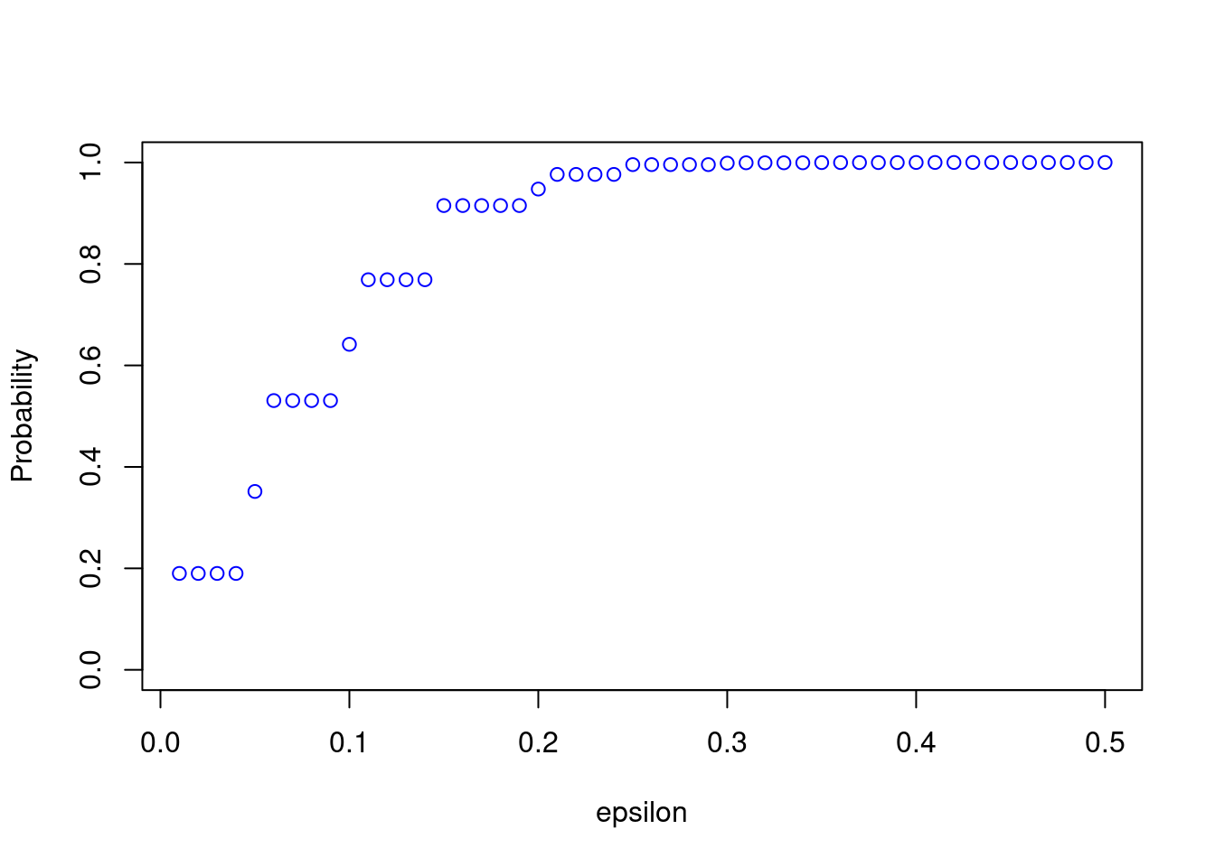
We can see from the plot that \(P\left( \mid \widehat\theta_n - \theta\mid < \varepsilon\right)\)is quite small for small values of \(\varepsilon\). Consistency means that for any \(\varepsilon>0\), the probability approaches \(1\) as \(n\rightarrow\infty\). We can now easily change the sample size and see how the results change. For example, take \(n=200\):
probs <- calc_probs_consistency(n = 200, S = 10000, p = 0.7, all_eps = seq(0.01, 0.5, by= 0.01))
plot(all_eps,probs,ylim = c(0,1),xlab="epsilon",ylab="Probability", col = 'blue')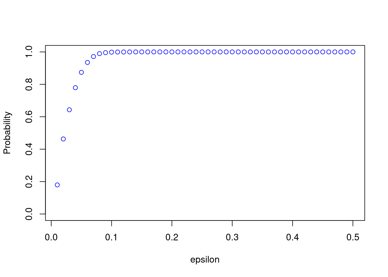
5.4 Asymptotic Normality
We know from the Central Limit Theorem that \[ \frac{\sqrt{n}\left(\overline X_n - E(X)\right)}{s_n} \rightarrow_D N(0,1), \] where \(s_n\) is the sample standard deviation. Convergence in distribution means that the distribution of the normalized sample average converges to the distribution function of a standard normal random variable.
Again, we can use the previous simulation setup to illustrate this property. To do so, we calculate
\[ P\left(\frac{\sqrt{n}\left(\overline X_n - E(X)\right)}{s_n} \leq z\right) \] and compare it to the standard normal cdf evaluated at z. We then plot the results as a function of z. Just as before, we define a function that calculates the probabilities:
calc_probs_asymp_normal <- function(n,S,p,z) {
  n_z = length(z)
  X <- replicate(S,rbinom(n,1,p))
  theta_hat <- colMeans(X)
  stds <- apply(X, 2, sd)
  probs = rep(0, n_z)
  for (i in 1:n_z) {
    probs[i] = mean( sqrt(n)*(theta_hat - p)/stds <= z[i])
  }
  return(probs)
}
We can now plot the results for different sample sizes such as
z = seq(-3,3,by=0.01)
probs <- calc_probs_asymp_normal(n = 20, S = 10000, p = 0.7, z = z)
plot(z,probs,ylim = c(0,1),xlab="z",ylab="Probability", col = 'blue')
lines(z, pnorm(z, 0, 1), col = 'red',lwd = 2)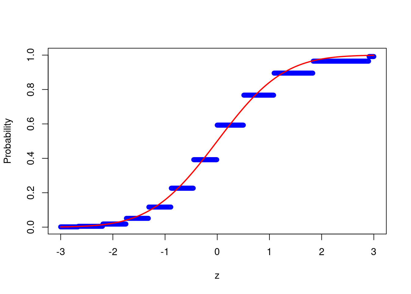 or
or
probs <- calc_probs_asymp_normal(n = 2000, S = 10000, p = 0.7, z = z)
plot(z,probs,ylim = c(0,1),xlab="z",ylab="Probability", col = 'blue')
lines(z, pnorm(z, 0, 1), col = 'red',lwd = 2)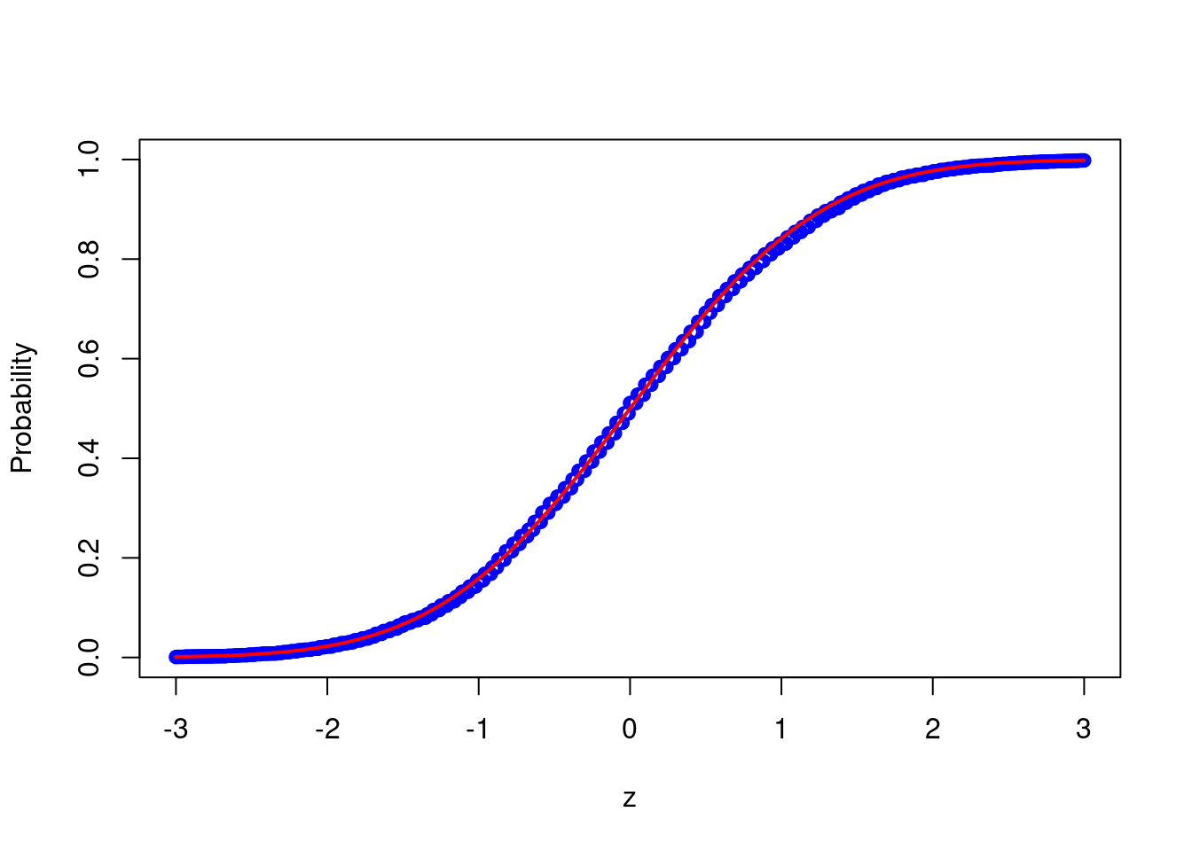
5.5 Testing
Let \(\{X_1,X_2,…,X_n\}\) be a random sample and define \(\mu=E(X)\). Suppose we want to test \(H_0:\mu=\mu_0\) where \(\mu_0\) is a fixed number. To do so, define \[ t_n = \frac{\sqrt{n}\left(\overline X_n - \mu_0\right)}{s_n}. \] An immediate consequence of the Central Limit Theorem is that if \(H_0\) is true then \[ t_n = \frac{\sqrt{n}\left(\overline X_n - \mu_0\right)}{s_n} = \frac{\sqrt{n}\left(\overline X_n - \mu\right)}{s_n} \rightarrow_D N(0,1) \]
and therefore \[ \underset{n \rightarrow \infty}{\lim}P\left(\mid t_n\mid>1.96 \mid \mu = \mu_0\right) = 0.05. \]
Hence, if we reject when \(|t_n|>1.96\), we only reject a true null hypothesis with probability approaching \(5\%\).
If the null hypothesis is false, we can write \[ t_n = \frac{\sqrt{n}\left(\overline X_n - \mu_0\right)}{s_n} = \frac{\sqrt{n}\left(\overline X_n - \mu\right)}{s_n} + \frac{\sqrt{n}\left(\mu - \mu_0\right)}{s_n}. \] It follows now from \(\underset{n \rightarrow \infty}{\lim}\sqrt{n}|\mu - \mu_0| = \infty\) that \[ \underset{n \rightarrow \infty}{\lim} P\left(|t_n| > 1.96 | \mu \neq \mu_0\right) = 1, \]
i.e. we reject a false null hypothesis with probability approaching 1. However, for a small sample size, the rejection probability is typically much smaller when \(\mu_0\) is close to \(\mu\).
Therefore, we want to calculate the small sample rejection probabilities using Monte Carlo simulations. We could either vary \(μ_0\) (the value we test) or \(\mu\) (the true mean). We take the latter because you will see power functions using this approach later in class as well.
We work with the Bernoulli distribution again and define a function that calculates certain rejection probabilities.
calc_rej_probs <- function(n,S,mus,mu0,alpha) {
  n_mus = length(mus)
  probs = rep(0, n_mus)
  for (i in 1:n_mus) {
    X <- replicate(S,rbinom(n,1,mus[i]))
    theta_hat <- colMeans(X)
    stds <- apply(X, 2, sd)
    probs[i] = mean(abs( sqrt(n)*(theta_hat - mu0)/stds ) > qnorm(1-alpha/2) )
  }
  return(probs)
}
We can now call the function for different values of \(\mu\) and plot the rejection probabilities
mus = seq(0.5,0.9,by=0.01)
probs <- calc_rej_probs(n = 200, S = 10000, mus = mus, mu0 = 0.7, alpha = 0.05)
plot(mus,probs,ylim = c(0,1),xlab="True mean",ylab="Rejection Probability", col = 'blue')
abline(h=0.05, col = 'red',lwd = 2)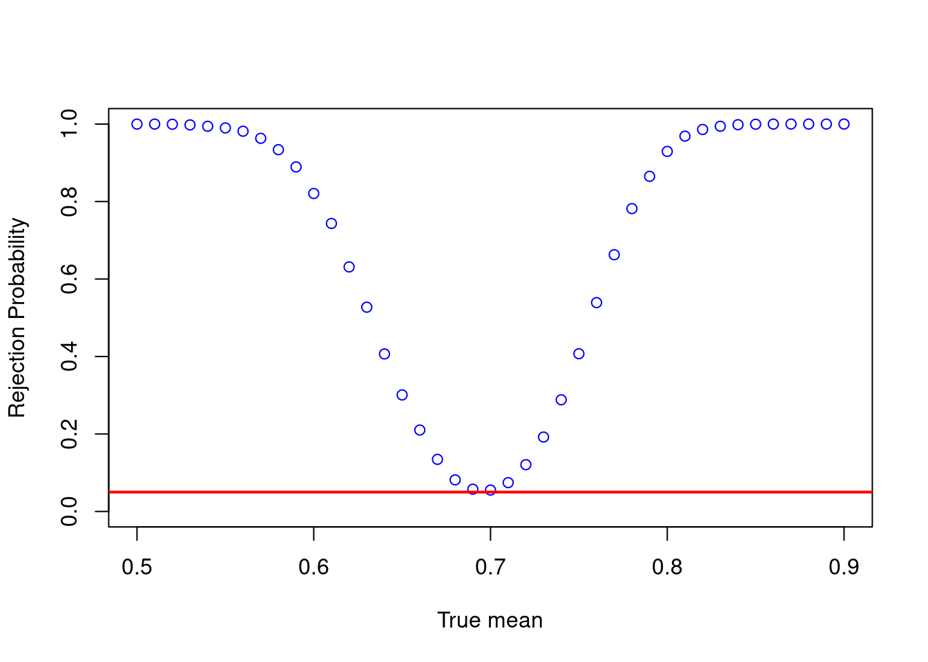
5.6 Parallel Computing
In the following we will shortly discuss how we can speed up our Monte Carlo simulations. So far we only considered very simple examples that didn’t take much time. During your future research projects the R-Code might become more complex such that the simulations will need more computing time. Most computers have nowadays more than one core and that is helpful for Monte Carlo simulations. As we repeat one task several times we can distribute the different tasks to different cores such that the code can be executed in parallel. R offers some easy ways to to do that. Here, we will consider two examples.
First of all we need to load the packages parallel, foreach and doParallel. We need the package parallel as it contains the functions makeCluster() and parLapply(). From the package foreach we use the function foreach() and from doParallel the function registerDoParallel().
## Loading required package: iteratorsIn the first Monte Carlo simulation we use the function foreach() that works as a for-loop. Here, we create a matrix X = replicate(S,rbinom(n,1,0.7)) where S=10,000 and n = 1000. It takes some time to do this operation and we will repeat this \(50\) times. Therefore, we will see that it makes sense to distribute the tasks to several cores.
S = 10000
n = 1000

t1 = Sys.time()
out1 = foreach(i=1:50) %do%{
              X = replicate(S,rbinom(n,1,0.7))
              I = rep(1,n)
              XX = mean(I%*%X)/n       # make sure that calculating the mean in this way is inefficient. Just use mean(X)
              XX
        }
t2 = Sys.time()
t2 - t1
## Time difference of 17.09851 secsIn the second step we replace %do% by %dopar% in the foreach() function. This enables us to use more than one core. We use 4 cores here. We need to tell R that we want to use more than one core with registerDoParallel(4).
#load cluster
np = 4                                         # number of cores used
cl = registerDoParallel(np)
t1 = Sys.time()
out1 =  foreach(i=1:50) %dopar%{
              X = replicate(S,rbinom(n,1,0.7))
              I = rep(1,n)
              XX = mean(I%*%X)/n
              XX
        }
t2 = Sys.time()
t2 - t1
## Time difference of 5.361912 secsAs we can see, doing the calculation in parallel speeds the code up.
A second possible way to use more than one core is to use the function parLapply() that is a multicore version of lapply(). In order to use lapply() we need to define a function, where \(i\) is just an index as in the foreach() function. Note that \(i\) needs to be the first variable of the defined function.
Test = function(i,n,S){
                X = replicate(S,rbinom(n,1,0.7))
                I = rep(1,n)
                XX = mean(I%*%X)/n
                XX
            }
t1 = Sys.time()
out3 = lapply(1:50, Test,n = n, S = S)
t2 = Sys.time()
t2 - t1
## Time difference of 16.86668 secsOnce again we need to tell R that we want to use more than one core and we do use this in case of parLapply() with makeCluster(4). Make sure to stop the cluster with stopCluster() when you do not need it anymore.
cl2 <- makeCluster(np)                          # set up cores
t1 = Sys.time()
out4 = parLapply(cl2, 1:50, Test,n=n,S=S)
t2 = Sys.time()
t2 - t1
## Time difference of 5.48056 secsAs we can see the operation is faster here as well. There exist many other ways to execute code in parallel in R. Depending on the situation the one or the other might be preferable.