Chapter 3 The k-NN Algorithm
It is easiest to illustrate the nearest neighbor method (k-NN, for short) with an example.
A microfinance institute in Africa makes loans available to starting entrepreneurs.
Until now, loan applications have been mainly processed and assessed by field workers (loan officers) who visit villages.
About 40% of the applications are approved.
The field workers have gained a lot of experience over time and are able to make an educated guess on whether clients are able to pay the interest and repay the loan (over 90% of the loans are repaid on time).
However, with the introduction of mobile technology, an increasing number of applications reach the head offices directly, and are assessed by administrative staff who have no direct contact with the applicants.
The head office has a wealth of data on loans granted and rejected, and on characteristics of the applicants.
The challenge is to find out if it's possible to determine whether a loan should be granted or not, on the basis of a number of simple characteristics (including age, gender, experience).
3.1 Distance, and Similarity
New applicants can be compared with "similar" applicants from the past.
If a loan has been granted to the majority of that set, then we also grant the loan to the new applicant (and reject the loan otherwise).
The set of similar applicants is determined by a number of characteristics that we believe are relevant.
Ten characteristics have been selected from the data on the application form:
- Gender (a dummy variable: 0 = female; 1 = male)
- Age (in years)
- Experience (number of years working, self-employed or in paid employment)
- Own assessment of entrepreneurial skills (a 10-point scale; 1 = very poor; 10 = excellent)
- Been self-employed in the past (0 = no; 1 = yes)
- Education level (1 = none; 2 = primary education; 3 = secondary education; 4 = university)
- Parent education level (same coding)
- In possession of a savings account (0/1)
- Living in the city or countryside (0 = countryside; 1 = city)
- Marital status (0 = not married; 1 = married).
Discussions with field workers have shown that these characteristics are relevant, but in an often quite complex way.
Older applicants bring more experience, which is positive.
At the same time, older applicants often lack the energy to successfully start something new, especially if they have not had a business before.
Younger entrepreneurs have no experience but have better skills (such as knowledge of IT).
Education level is a good indication especially if it is higher than that of the parents (it indicates perseverance and commitment).
In short, the decision whether or not to allocate a loan is complex and, moreover, at least partly intuitive.
When a new applicant registers, we will compare his or her data with the applicants from the past.
We search the database for applicants with similar characteristics. We may find applicants with exactly the same characteristics. The distance between the new applicant and the existing customer then is zero.
The distance between two people is determined on the basis of the differences in the ten characteristics.
You can compute he distance in a variety of ways.
- You can measure the absolute differences, and then sum them over the 10 characteristics.
- But mostly we use the so-called Euclidean distance.
We work in three steps.
- In the first step, we determine the squared differences between two objects (or, as in our example, people).
- In the second step, we add up all (in our example, ten) squared differences.
- And, finally, in step 3, we will take the square root of the result of step 2.
Note: this is actually an extension of the Pythagorean theorem that you probably remember from high school!
The straight-line distance between two points can be calculated as the square root of the sum of the squared differences in horizontal and vertical directions. The extension is that we now have more than two dimensions.
3.2 Normalize or Standardize Data
When calculating distances, we have to take into account the units used.
Age is expressed in years, and the range of measurements (the highest observed age minus the lowest observed age) in our customer base can be as high as 40 (years).
For gender we use a (0/1) dummy variable that gives 1 as the maximum difference.
If we also included the amount in the savings account as a characteristic, the value (in units of local currency) could run in the thousands or even millions.
The problem of different and incomparable units can be solved in two ways: by normalization, or by standardization.
3.3 Normalizing Data
Normalization is the recalculation of the data to values between 0 (the minimum) and 1 (the maximum) with the formula:
xn = (x - xmin)/ xmax - xmin)
For example, if age ranges from 20 to 50, then an applicant aged 35 has a normalized age of
xn = (35-20) / (50-20) = 0.50 (halfway between the lowest and highest age observed).
Normalizing variables makes them comparable. Computing distances for non-normalized data, in effect assigns higher weights to variables with wider ranges of values.
Self Test You are in a class of 20 students. Your grade for this module is 7. The grades of your class range from 4 (minimum) to 9 (maximum). What is your normalized score for the exam?
3.4 Standardizing Data
An alternative to normalization is standardization.
Here we determine the Z-scores of the data, assuming the data are normally distributed.
The Z scores are negative (positive) for values smaller (larger) than the mean.
Standardization is preferable to normalization if the criteria are unbounded (e.g., ranging from 0 to ∞) and/or there are outliers in either direction (e.g., very low or high incomes, compared to the rest of the group).
Whichever the choice, outliers tend to have an impact on your analysis, and it pays off to somehow deal with this issue! If the outlier reflects an error, then obviously it has to be corrected. If the outlier is not representative of the population (Bill Gates applying for a microloan), then deleting it is an option. Recoding very high values to a predetermined maximum might also work. In general: try to see how sensitive your analysis is to different methods!!
Suppose all persons in your data set earn between 0 and 100 monetary units, except for one person who earns 10,000. The bulk of the normalized values would then be between 0 and 0.01, and have little weight in finding nearest neigbours.
3.5 Choosing the Number of Neighbors (k)
Oh yes, it's k-NN, not NN! Let's turn our attention to k!
The k signifies the number of nearest neighbours we want to analyze.
The outcome of the algorithm is sensitive to the choice of k.
If we set k very large, then it becomes ever more likely that the majority in the dataset will dominate.
In our case, since the majority of applications are rejected, the likelihood of a majority of rejections increases as k increases.
In the extreme case, with k as large as the data set, we reject all applications because the majority of applications in the past was rejected! But if the bank rejects all applications, then it will cease to exist. That's not what we want.
If, on the other hand, we choose a very small k (in the extreme case, k=1) we run the risk that small groups that may be uncorrectly labeled will have an undesirably large influence on the predictions.
For example, a person with extreme scores on, say, age and entrepreneurial skills, who got a loan but really shouldn't have gotten it, has an undue influence on the predictions of new applicants with the same characteristics.
So, we have to find some optimum, in between these extremes.
As a rule of thumb, we often use the square root of the number of observations.
For example, for 500 observations, we would set k to √500 = 22. In the case of a binary classification (a classification into two groups), however, we prefer an odd number so that there is always a majority; we can set k to 21 or 23.
This is just a rule of thumb. To make the model as good as possible, we will experiment with the value of k!
3.6 Application of k-NN in R
Let's apply the k-NN algorithm step by step to an example.
The steps are as follows.
- Reading and describing the data
- Preparing the data for application of the k-NN algorithm:
- Normalize (or standardize) the data
- Splitting the data into a training set and a test set
- Training the model on the data
- Evaluating the model
- Improving the model.
3.6.1 Step 1: Reading and Describing the Data
We are going to work in an R-script.
Our data comes from a STATA file (ML3_1_KNN.dta) that we can read with read.dta().
To use this function we must first load the package foreign, with library(foreign).
We read the file as a data frame called knndata.
We can look at the structure of that file with the str() command.
library(foreign)
knndata<-read.dta("ML3_1_KNN.dta",convert.factors=FALSE)
str(knndata)
## 'data.frame': 500 obs. of 13 variables:
## $ id : num 1 2 3 4 5 6 7 8 9 10 ...
## $ male : num 1 0 0 0 0 1 0 1 0 0 ...
## $ age : num 49 29 40 33 27 40 46 46 25 32 ...
## $ exp : num 2 1 20 12 1 8 21 2 7 1 ...
## $ skills : num 3 1 10 10 10 10 1 10 10 10 ...
## $ busexp : num 0 0 1 0 0 0 1 0 0 0 ...
## $ educ : num 1 1 1 1 2 3 3 2 2 1 ...
## $ educpar: num 1 1 1 1 4 2 4 2 4 1 ...
## $ saving : num 0 0 0 0 0 0 1 0 1 0 ...
## $ city : num 0 1 0 0 1 1 0 0 0 0 ...
## $ marital: num 1 0 1 1 1 0 1 1 0 1 ...
## $ savacc : num 6.28 14.37 11.51 5.16 17.86 ...
## $ accept : num 0 0 1 0 0 0 1 1 0 1 ...
## - attr(*, "datalabel")= chr ""
## - attr(*, "time.stamp")= chr "14 Apr 2016 11:56"
## - attr(*, "formats")= chr [1:13] "%9.0g" "%9.0g" "%9.0g" "%9.0g" ...
## - attr(*, "types")= int [1:13] 254 254 254 254 254 254 254 254 254 254 ...
## - attr(*, "val.labels")= chr [1:13] "" "" "" "" ...
## - attr(*, "var.labels")= chr [1:13] "" "" "" "" ...
## - attr(*, "version")= int 12From the output we see that the data frame has 500 observations and 13 variables.
The values of the first records in the data frame are displayed.
Before we get started, we still have to do the necessary preliminary work.
- Some variables are not needed for the analysis (id; savacc).
- The variable id is a serial number of the records in the file and does not contain useful information.
- The variable savacc is an estimated amount of the applicant's savings. Because the savings balance is only a snapshot, the loan officers look at having a savings account or not as an indication, rather than the savings balance.
- The variable that we call the label in the k-NN method must be a factor variable. The label here is accept, but it is a numeric variable.
- We have to check that all variables have values in the expected range (no ages above 80 or below 16; all dummies are indeed 0 or 1; the entrepreneurial skills are on a 10-point scale with values from 1 to 10; and so on).
3.6.1.1 Selection and Description of Variables
First of all, we select the variables to be used in our analysis.
There are several ways to do this.
It is good practice to position the label variable that indicates the group the object (or person) belongs to in the first column. Our label variable (accept) is now in the last of the 13 columns.
We do not need the variables id and savacc.
First we create a new factor variable, acceptFac, from the numeric variable accept, with the factor() function.
In that function we can indicate:
- what the values (levels) are in the original variable, and
- how we want to label those values.
We can describe the new variable with the self-written CFR() function introduced in the previous chapter.
knndata$acceptFac <- factor(knndata$accept, levels=c(0,1),
                     labels=c("Reject","Accept"))
round(100*table(knndata$acceptFac)/length(knndata$acceptFac),0)
##
## Reject Accept
## 61 39Indeed, around 60% (61%, to be more precise) of the 500 applications were rejected.
Now that we have the new variable acceptFac we can create a new file with only the required variables, and acceptFac in the first column 1.
With the head() function we display the first (6) observations, and summary() gives a description of all variables.
Always study the output carefully: any coding errors or outliers will quickly come to light! This file does not appear to contain any coding errors or strange values. The coding for education level is as expected from 1 to 4; ages range from 21 to 50; and so on.
knndata2 <- knndata[,c("acceptFac","male","age","exp","skills",
                       "busexp","educ","educpar","saving",
                       "city","marital")]
head(knndata2)
## acceptFac male age exp skills busexp educ educpar saving city marital
## 1 Reject 1 49 2 3 0 1 1 0 0 1
## 2 Reject 0 29 1 1 0 1 1 0 1 0
## 3 Accept 0 40 20 10 1 1 1 0 0 1
## 4 Reject 0 33 12 10 0 1 1 0 0 1
## 5 Reject 0 27 1 10 0 2 4 0 1 1
## 6 Reject 1 40 8 10 0 3 2 0 1 0summary(knndata2)## acceptFac male age exp skills
## Reject:304 Min. :0.000 Min. :21.00 Min. : 0.000 Min. : 1.000
## Accept:196 1st Qu.:0.000 1st Qu.:29.00 1st Qu.: 4.000 1st Qu.: 1.000
## Median :0.000 Median :37.00 Median : 8.000 Median : 3.000
## Mean :0.412 Mean :35.98 Mean : 9.214 Mean : 5.224
## 3rd Qu.:1.000 3rd Qu.:43.00 3rd Qu.:13.000 3rd Qu.:10.000
## Max. :1.000 Max. :50.00 Max. :30.000 Max. :10.000
## busexp educ educpar saving city
## Min. :0.000 Min. :1.000 Min. :1.00 Min. :0.000 Min. :0.000
## 1st Qu.:0.000 1st Qu.:1.000 1st Qu.:1.00 1st Qu.:0.000 1st Qu.:0.000
## Median :0.000 Median :2.000 Median :2.00 Median :0.000 Median :0.000
## Mean :0.232 Mean :2.016 Mean :2.16 Mean :0.244 Mean :0.498
## 3rd Qu.:0.000 3rd Qu.:3.000 3rd Qu.:3.00 3rd Qu.:0.000 3rd Qu.:1.000
## Max. :1.000 Max. :4.000 Max. :4.00 Max. :1.000 Max. :1.000
## marital
## Min. :0.000
## 1st Qu.:0.000
## Median :1.000
## Mean :0.614
## 3rd Qu.:1.000
## Max. :1.0003.6.2 Step 2: Preparing the Data
3.6.2.1 Normalizing the Data
The k-NN method - like most methods for clustering objects - is based on distances between objects.
However, we are dealing with variables that are expressed in different units.
- There are dummy variables that take on value of 0 or 1
- age is expressed in years (with a maximum of 50)
- skills is measured on a 10-point scale
- educational level (educ) is measured on a 4-point scale.
To bring all variables to the same level, we can either normalize or standardize them.
Often we use normalization based on the value of an object on a scale that runs from 0 (the minimum value of the variable) to 1 (the maximum). The normalized values always lie between 0 and 1, which is a nice feature.
Note that the dummy variables in this method remain unchanged!
We can determine the normalized value for each variable separately.
For example for age we can write the following lines:
# Example: normalizing age
knndata2$age_n <- (knndata2$age-min(knndata2$age))/(max(knndata2$age)-min(knndata2$age))
head(knndata2[,c("age","age_n")])
## age age_n
## 1 49 0.9655172
## 2 29 0.2758621
## 3 40 0.6551724
## 4 33 0.4137931
## 5 27 0.2068966
## 6 40 0.6551724Just to check, someone of 29 years old has a normalized age of \((29-21)/(50-21) = 0.2759\).
This method requires a lot of typing, and is very error-prone. Whenever things are repetitive, consider writing a function!
We will write a function called normalizer().
# normalize data
normalizer <- function(x){
  return((x-min(x))/(max(x)-min(x)))
}
The normalizer() function is defined as an object.
Once run, the function will appear as an object in your top right screen, in RStudio.
Between the brackets "{" and "}", is stated what the function does.
We normalize the argument (x) of the function, with a simple formula that makes use of standard functions in R, namely max() and min().
We can now apply the function to the 10 variables in our file.
We cannot and should not normalize the label variable: it's a factor variable which cannot be normalized!
This all can be done in one step by applying the function to a list of data. A data frame is in fact a list of vectors pasted together.
To apply operations to a list, we use lapply() function.
We write the normalized data in a new data frame knndata2_n. Note again that we leave out the first column (the label variable: accept or reject).
# Normalized data; leave out the label variable acceptFac (in the first column)
knndata2_n <- as.data.frame(lapply(knndata[,2:11], normalizer))
summary(knndata2_n)
## male age exp skills
## Min. :0.000 Min. :0.0000 Min. :0.0000 Min. :0.0000
## 1st Qu.:0.000 1st Qu.:0.2759 1st Qu.:0.1333 1st Qu.:0.0000
## Median :0.000 Median :0.5517 Median :0.2667 Median :0.2222
## Mean :0.412 Mean :0.5164 Mean :0.3071 Mean :0.4693
## 3rd Qu.:1.000 3rd Qu.:0.7586 3rd Qu.:0.4333 3rd Qu.:1.0000
## Max. :1.000 Max. :1.0000 Max. :1.0000 Max. :1.0000
## busexp educ educpar saving
## Min. :0.000 Min. :0.0000 Min. :0.0000 Min. :0.000
## 1st Qu.:0.000 1st Qu.:0.0000 1st Qu.:0.0000 1st Qu.:0.000
## Median :0.000 Median :0.3333 Median :0.3333 Median :0.000
## Mean :0.232 Mean :0.3387 Mean :0.3867 Mean :0.244
## 3rd Qu.:0.000 3rd Qu.:0.6667 3rd Qu.:0.6667 3rd Qu.:0.000
## Max. :1.000 Max. :1.0000 Max. :1.0000 Max. :1.000
## city marital
## Min. :0.000 Min. :0.000
## 1st Qu.:0.000 1st Qu.:0.000
## Median :0.000 Median :1.000
## Mean :0.498 Mean :0.614
## 3rd Qu.:1.000 3rd Qu.:1.000
## Max. :1.000 Max. :1.000The output of summary() confirms that the normalizer() function does what it is supposed to do: the minima and maxima of all variables are now all 0 and 1. The variables are now expressed in comparable units. Or unit-free, if you prefer.
Normalizing is an important step. The software will also work with data that has not been normalized without any warning. But the variables with the greatest range (here age) then carry much more weight, and that's probably not what we want. Computers are smarter than you think. But never smarter than you are.
3.6.2.2 Splitting the Data into a Training Set and a Test Set
The next step is to split the data into a training and a test set.
With the training set we want to develop a model that predicts grouping (accept or reject) based on the 10 criteria that we suspect are important.
But we must determine whether the model works properly on a test set of data not used in the development of the model.
An recurring question is the size of the two sets.
On the one hand, we naturally want to use as much information as possible to determine the best possible model.
But at the same time, we want to have a test set that is large enough to make statistically sound statements about the predictive power of the model.
Commonly used rules of thumb are to use 20% or 25% of the data set for testing the model. But with very large data sets, that percentage can be adjusted downwards.
Another issue is how to split the data into a training and a test set.
If the data are in random order then we can simply use the first 80% of the records for the training set and the last 20% for the test set. But if the data is sorted in some way (for example by age, or by the label variable) then it is very unwise to follow this method. In general it is better to take a random sample from the data file.
Often, we are not entirely sure of how the data are organized. So, a random sample is recommended!
Drawing a sample is done as follows.
We know that the data file has about 500 records (but we can let R do the work with the nrow() function).
For convenience, we want to have a test set of exactly 100 records.
Functions dealing with samples and random numbers, are actually not truly random: based on a certain starting point (indicated by a number that we call seed) the result of the drawings is fixed. This is often useful, because results can be reproduced with that information.
The starting point we chose with set.seed() is 123. Running set.seed(12321) produces the same results as described below. Using a different starting point, or not running set.seed() at all, gives different results. However, if the sample is large enough, the conclusions are bound to be the same.
The sample stored in the vector train_steekproef is a set of 400 unique numbers. The size of our file turns out to be 500 (from the nrow() function), and we ourselves determined that the test set must have a size of 100 records.
set.seed(123)              # for reproducibility of the results!
x <- nrow(knndata2_n)        # determine number of observations (500)
train_set <- sample(x,x-100) # sample a training set (and leave 100 for testing)
str(train_set)               # show me the structure of the training set
## int [1:400] 415 463 179 14 195 426 306 118 299 229 ...# use the vector to split our data
# this must be applied to both the criteria and the label variable!
knn_train <- knndata2_n[train_set,]
knn_test <- knndata2_n[-train_set,]
knn_train_label <- knndata2[train_set, 1]
knn_test_label <- knndata2[-train_set, 1]
str(knn_train)## 'data.frame': 400 obs. of 10 variables:
## $ male : num 0 0 0 0 1 0 1 1 1 0 ...
## $ age : num 0.207 0.586 0.414 0.828 0.931 ...
## $ exp : num 0.267 0.2 0.433 0.133 0.8 ...
## $ skills : num 1 0 0 0 0.222 ...
## $ busexp : num 0 0 1 0 1 0 1 0 1 0 ...
## $ educ : num 0.333 0 0 0 0.667 ...
## $ educpar: num 0.333 0 0 0 0 ...
## $ saving : num 0 0 0 0 0 1 1 1 0 0 ...
## $ city : num 0 1 0 0 0 0 1 0 1 0 ...
## $ marital: num 0 1 1 1 1 1 1 0 1 1 ...str(knn_test)## 'data.frame': 100 obs. of 10 variables:
## $ male : num 1 0 1 1 0 0 1 1 1 1 ...
## $ age : num 0.966 0.31 0.31 0.552 0.793 ...
## $ exp : num 0.0667 0.1 0.3 0.1333 0.8 ...
## $ skills : num 0.222 0 1 0.111 1 ...
## $ busexp : num 0 0 0 0 1 0 0 0 1 1 ...
## $ educ : num 0 0 1 0 0 ...
## $ educpar: num 0 0 0.333 0 0 ...
## $ saving : num 0 0 1 0 0 1 0 0 0 0 ...
## $ city : num 0 0 1 1 0 0 1 1 0 0 ...
## $ marital: num 1 0 0 1 1 1 0 1 1 1 ...str(knn_train_label); length(knn_train_label)## Factor w/ 2 levels "Reject","Accept": 1 1 1 1 2 2 2 1 2 1 ...## [1] 400str(knn_test_label) ; length(knn_test_label)## Factor w/ 2 levels "Reject","Accept": 1 1 1 1 2 2 1 1 1 2 ...## [1] 1003.6.3 Step 3: Training the Model
We use the package class to train the model with the k-NN method.
First, if you haven't already done so, install the package with install.packages(“class”), and then load the functions of the package with library(class).
Note: in RStudio you will find all available packages under the “Packages” tab. Some of these you have installed yourself, while others are already available in the system. The packages you have installed yourself are in the user library, and the packages available within the system are in the system library. Depending on the version of R you are using, some packages fall into the second category. In recent versions of R, popular packages like foreign and class are already in the system library, which means that you do not need to install using install.packages(). But installing won't hurt. Search for class yourself, and click on the package to learn more about the package and its functions! Packages in the system library too must be invoked using the library() command!
We use the knn() function to train the model.
In parentheses we put:
- the training set
- the test set, and
- the labels (or groupings) in the training set)
- the number of neigbours.
We already have created the files needed.
We must indicate how many nearest neigbours (k) to be be used in determining the predicted grouping.
As a rule of thumb, a good first choice is the square root of the number of records. We want to avoid a situation in which the algorithm cannot make a decision because the same number of nearest neigbours fall in the two groups, by choosing an odd number.
In our example, the square root of 500 is (rounded) 22. In rare cases, 11 of the 22 nearest neigbours may have been accepted and 11 rejected, so that group allocation must be made randomly. We can easily avoid this situation by setting k1 to 21 or 23.
But let's ask R to do the job for us!
library(class)## Warning: package 'class' was built under R version 4.0.3# choice of k: odd number close to square root of number of observations
k1 <- round(sqrt(nrow(knndata2_n)))
k1 <- ifelse(k1%%2==0, k1-1,k1)
cat("Our choice for k is:", k1,"[ = odd number, close to square root of",x,"]\n")## Our choice for k is: 21 [ = odd number, close to square root of 500 ]knn_pred <- knn(train=knn_train, test=knn_test, cl=knn_train_label, k1)
knn_pred## [1] Reject Reject Reject Reject Accept Accept Reject Reject Reject Reject
## [11] Accept Reject Reject Reject Reject Accept Accept Reject Accept Accept
## [21] Accept Accept Reject Reject Accept Reject Accept Accept Reject Accept
## [31] Reject Reject Reject Reject Accept Reject Accept Accept Reject Reject
## [41] Reject Accept Accept Accept Accept Accept Reject Reject Reject Reject
## [51] Reject Reject Reject Reject Accept Reject Accept Reject Reject Reject
## [61] Accept Accept Reject Reject Reject Reject Reject Accept Accept Accept
## [71] Accept Reject Reject Reject Reject Reject Reject Reject Reject Accept
## [81] Reject Reject Accept Reject Accept Reject Accept Reject Accept Accept
## [91] Accept Reject Reject Reject Reject Reject Accept Reject Accept Reject
## Levels: Reject Accept3.6.4 Step 4: Evaluate the Model
For the evaluation of the model we are interested in the actual value and the predicted value in the test set.
Since we have a dichotomy (accept or reject), there are four possibilities:
- Correctly predicted acceptance
- A correctly predicted rejection
- A rejection that is incorrectly predicted as acceptance
- An acceptance incorrectly predicted as rejection.
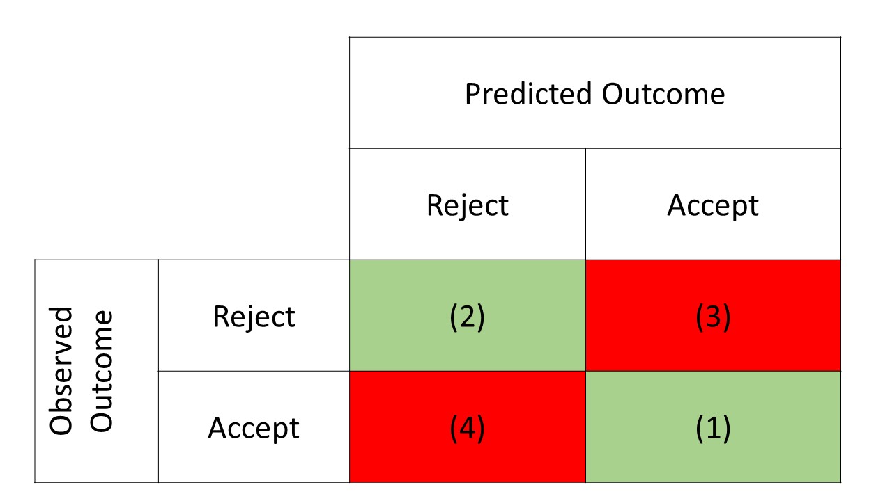
The green shaded cells in the table represent the correct predictions, and the red shaded cells represent the incorrect predictions.
A first test for the value of the model is the sum of the first two categories (the green shaded cells): what percentage of the records in the test set is correctly classified by the model?
But - unless the model predicts 100% correctly - we also have to look at the last two categories separately.
It is quite conceivable that one error category is more serious than the other.
In our example: it may be more costly to wrongly allocate a loan (the bank will then have lost all the money) than to wrongly reject a loan (the bank will then only miss out on the profit on a loan).
What's worse, of course, is up to the ultimate decision maker, and not so much to the analyst.
R can create simple tables with, for example, table().
For nicer tables with more information we can use the functions in get gmodels package.
Assuming the package is already installed we can do the following.
library(gmodels)## Warning: package 'gmodels' was built under R version 4.0.4CrossTable(knn_test_label,knn_pred,chisq=TRUE, expected=TRUE, format="SPSS")##
## Cell Contents
## |-------------------------|
## | Count |
## | Expected Values |
## | Chi-square contribution |
## | Row Percent |
## | Column Percent |
## | Total Percent |
## |-------------------------|
##
## Total Observations in Table: 100
##
## | knn_pred
## knn_test_label | Reject | Accept | Row Total |
## ---------------|-----------|-----------|-----------|
## Reject | 57 | 5 | 62 |
## | 38.440 | 23.560 | |
## | 8.961 | 14.621 | |
## | 91.935% | 8.065% | 62.000% |
## | 91.935% | 13.158% | |
## | 57.000% | 5.000% | |
## ---------------|-----------|-----------|-----------|
## Accept | 5 | 33 | 38 |
## | 23.560 | 14.440 | |
## | 14.621 | 23.856 | |
## | 13.158% | 86.842% | 38.000% |
## | 8.065% | 86.842% | |
## | 5.000% | 33.000% | |
## ---------------|-----------|-----------|-----------|
## Column Total | 62 | 38 | 100 |
## | 62.000% | 38.000% | |
## ---------------|-----------|-----------|-----------|
##
##
## Statistics for All Table Factors
##
##
## Pearson's Chi-squared test
## ------------------------------------------------------------
## Chi^2 = 62.05909 d.f. = 1 p = 3.33305e-15
##
## Pearson's Chi-squared test with Yates' continuity correction
## ------------------------------------------------------------
## Chi^2 = 58.76042 d.f. = 1 p = 1.780876e-14
##
##
## Minimum expected frequency: 14.44In the table, the actual grouping is broken down by the predicted score.
- Of the 66 records that were rejected in practice, 63 were correctly predicted by kNN model; 3 rejected applications were incorrectly predicted as accepted.
- Of the 34 applications accepted, 23 are correctly predicted, so that the total number of correct predictions is 63 + 23 = 86. For the accepted applications, the number of incorrect predictions (11/34 = 32%) is quite high, but this can be perceived as less serious than the number of incorrectly accepted applications.
3.6.5 Step 5: improving the model
Within the framework of the data that we have available, there are a number of possibilities to improve the model.
Outside of the frameworks, we could think of collecting important extra information, or splitting the persons into more than two groups (in addition to rejection and acceptance, also a group of doubtful cases).
We can also see whether models with fewer variables work equally well (in that case we no longer need to ask applicants for redundant information).
Here, we are going to change two things:
- We are going to apply standardization instead of normalization.
- And we will change the number of nearest neighbors.
3.6.5.1 Standardization as an alternative
Standardization is a good option if some of the variables have skewed distributions and/or outliers.
In our data set there are no variables that lend themselves to this and the expected change in the result is therefore small.
We'll show it anyway for the sake of illustration.
For normalization we used the self-written normalize() function in combination with lapply().
For standardization, we hve the scale() function in R. The function can be applied to a data frame, and it works on each variable individually (that is, we don't need lapply()).
We leave the label variable unchanged, and for the samples (training and test sets) we also use the files that we have already created. It would not be wise to use different samples because changes in the results can then be due to random changes in the sample and not changes in the method!
# Standardized data (not for the "label" variabele acceptFac!!
knndata3_z <- as.data.frame(scale(knndata2[2:11]))
summary(knndata3_z)
## male age exp skills
## Min. :-0.8362 Min. :-1.8184 Min. :-1.3228 Min. :-0.9954
## 1st Qu.:-0.8362 1st Qu.:-0.8470 1st Qu.:-0.7486 1st Qu.:-0.9954
## Median :-0.8362 Median : 0.1243 Median :-0.1743 Median :-0.5241
## Mean : 0.0000 Mean : 0.0000 Mean : 0.0000 Mean : 0.0000
## 3rd Qu.: 1.1935 3rd Qu.: 0.8529 3rd Qu.: 0.5435 3rd Qu.: 1.1255
## Max. : 1.1935 Max. : 1.7028 Max. : 2.9842 Max. : 1.1255
## busexp educ educpar saving
## Min. :-0.5491 Min. :-1.01309 Min. :-1.0823 Min. :-0.5675
## 1st Qu.:-0.5491 1st Qu.:-1.01309 1st Qu.:-1.0823 1st Qu.:-0.5675
## Median :-0.5491 Median :-0.01595 Median :-0.1493 Median :-0.5675
## Mean : 0.0000 Mean : 0.00000 Mean : 0.0000 Mean : 0.0000
## 3rd Qu.:-0.5491 3rd Qu.: 0.98118 3rd Qu.: 0.7837 3rd Qu.:-0.5675
## Max. : 1.8176 Max. : 1.97832 Max. : 1.7168 Max. : 1.7585
## city marital
## Min. :-0.995 Min. :-1.2600
## 1st Qu.:-0.995 1st Qu.:-1.2600
## Median :-0.995 Median : 0.7921
## Mean : 0.000 Mean : 0.0000
## 3rd Qu.: 1.003 3rd Qu.: 0.7921
## Max. : 1.003 Max. : 0.7921Note that the means of all variables are indeed 0.
Standardized variables have a mean of 0 and a standard deviation of 1. With the sd() function you can verify that all standard deviations are indeed 1.
For example:
sd(knndata3_z$age)## [1] 1sd(knndata3_z$male)## [1] 1OK, let's go!
# de sampling vectors are still there ...
knn_train3 <- knndata3_z[train_set,]
knn_test3  <- knndata3_z[-train_set,]

str(knn_train3)
## 'data.frame': 400 obs. of 10 variables:
## $ male : num -0.836 -0.836 -0.836 -0.836 1.193 ...
## $ age : num -1.09 0.246 -0.361 1.096 1.46 ...
## $ exp : num -0.174 -0.461 0.544 -0.749 2.123 ...
## $ skills : num 1.126 -0.995 -0.995 -0.995 -0.524 ...
## $ busexp : num -0.549 -0.549 1.818 -0.549 1.818 ...
## $ educ : num -0.016 -1.013 -1.013 -1.013 0.981 ...
## $ educpar: num -0.149 -1.082 -1.082 -1.082 -1.082 ...
## $ saving : num -0.568 -0.568 -0.568 -0.568 -0.568 ...
## $ city : num -0.995 1.003 -0.995 -0.995 -0.995 ...
## $ marital: num -1.26 0.792 0.792 0.792 0.792 ...str(knn_test3)## 'data.frame': 100 obs. of 10 variables:
## $ male : num 1.193 -0.836 1.193 1.193 -0.836 ...
## $ age : num 1.581 -0.726 -0.726 0.124 0.974 ...
## $ exp : num -1.0357 -0.8921 -0.0307 -0.7486 2.1228 ...
## $ skills : num -0.524 -0.995 1.126 -0.76 1.126 ...
## $ busexp : num -0.549 -0.549 -0.549 -0.549 1.818 ...
## $ educ : num -1.01 -1.01 1.98 -1.01 -1.01 ...
## $ educpar: num -1.082 -1.082 -0.149 -1.082 -1.082 ...
## $ saving : num -0.568 -0.568 1.758 -0.568 -0.568 ...
## $ city : num -0.995 -0.995 1.003 1.003 -0.995 ...
## $ marital: num 0.792 -1.26 -1.26 0.792 0.792 ...knn_pred3 <- knn(train=knn_train3, test=knn_test3,cl=knn_train_label,k1)
CrossTable(knn_test_label,knn_pred3,chisq=TRUE, expected=TRUE, format="SPSS")##
## Cell Contents
## |-------------------------|
## | Count |
## | Expected Values |
## | Chi-square contribution |
## | Row Percent |
## | Column Percent |
## | Total Percent |
## |-------------------------|
##
## Total Observations in Table: 100
##
## | knn_pred3
## knn_test_label | Reject | Accept | Row Total |
## ---------------|-----------|-----------|-----------|
## Reject | 58 | 4 | 62 |
## | 38.440 | 23.560 | |
## | 9.953 | 16.239 | |
## | 93.548% | 6.452% | 62.000% |
## | 93.548% | 10.526% | |
## | 58.000% | 4.000% | |
## ---------------|-----------|-----------|-----------|
## Accept | 4 | 34 | 38 |
## | 23.560 | 14.440 | |
## | 16.239 | 26.495 | |
## | 10.526% | 89.474% | 38.000% |
## | 6.452% | 89.474% | |
## | 4.000% | 34.000% | |
## ---------------|-----------|-----------|-----------|
## Column Total | 62 | 38 | 100 |
## | 62.000% | 38.000% | |
## ---------------|-----------|-----------|-----------|
##
##
## Statistics for All Table Factors
##
##
## Pearson's Chi-squared test
## ------------------------------------------------------------
## Chi^2 = 68.92664 d.f. = 1 p = 1.021948e-16
##
## Pearson's Chi-squared test with Yates' continuity correction
## ------------------------------------------------------------
## Chi^2 = 65.44783 d.f. = 1 p = 5.967305e-16
##
##
## Minimum expected frequency: 14.44As expected, it doesn't matter whether we normalize or standardize.
3.6.5.2 Adjusted Values for k
The best value for k is a matter of trial and error.
At a high value for k, groups that are in some respect in the majority dominate, and the model adapts less flexibly to smaller groups.
With a low value for k, all kinds of exceptions (or incorrect coding) can have a major influence on the predictions.
Based on the rule of thumb that led to a choice k = 21, we can see whether predictions change systematically with changes in k. For example, we can choose values for k of 3, 5, 9, 15, 25 and 29 (always odd numbers).
All data sets are ready, and we can repeat the same command a number of times with new values for k each time.
It is more elegant to use a loop construction and to write easy-to-read output.
We take the number of correct predictions as the most important outcome.
The number of correct predictions is shown on the diagonal of the table: in the first row and first column, and in the second row and second column.
We can retrieve the numbers from the diagonal with the indices [1,1] and [2,2] of the table. The object corn is the number of correct rankings, and corp is the percentage.
With the cat() function we write the results in readable form.
# k=10
knn_pred <- knn(train=knn_train, test=knn_test,cl=knn_train_label,2)
CrossTable(knn_test_label,knn_pred,chisq=TRUE, expected=TRUE, format="SPSS")
##
## Cell Contents
## |-------------------------|
## | Count |
## | Expected Values |
## | Chi-square contribution |
## | Row Percent |
## | Column Percent |
## | Total Percent |
## |-------------------------|
##
## Total Observations in Table: 100
##
## | knn_pred
## knn_test_label | Reject | Accept | Row Total |
## ---------------|-----------|-----------|-----------|
## Reject | 56 | 6 | 62 |
## | 37.200 | 24.800 | |
## | 9.501 | 14.252 | |
## | 90.323% | 9.677% | 62.000% |
## | 93.333% | 15.000% | |
## | 56.000% | 6.000% | |
## ---------------|-----------|-----------|-----------|
## Accept | 4 | 34 | 38 |
## | 22.800 | 15.200 | |
## | 15.502 | 23.253 | |
## | 10.526% | 89.474% | 38.000% |
## | 6.667% | 85.000% | |
## | 4.000% | 34.000% | |
## ---------------|-----------|-----------|-----------|
## Column Total | 60 | 40 | 100 |
## | 60.000% | 40.000% | |
## ---------------|-----------|-----------|-----------|
##
##
## Statistics for All Table Factors
##
##
## Pearson's Chi-squared test
## ------------------------------------------------------------
## Chi^2 = 62.50707 d.f. = 1 p = 2.654893e-15
##
## Pearson's Chi-squared test with Yates' continuity correction
## ------------------------------------------------------------
## Chi^2 = 59.22644 d.f. = 1 p = 1.405326e-14
##
##
## Minimum expected frequency: 15.2tb<-table(knn_test_label,knn_pred); tb## knn_pred
## knn_test_label Reject Accept
## Reject 56 6
## Accept 4 34tb[2,2]## [1] 34kset <- c(3, 5, 9, 15, 21, 25, 29)
ssize <- 100
for (val in kset) {
knn_pred <- knn(train=knn_train, test=knn_test,cl=knn_train_label,val)
tb_true_neg <- table(knn_test_label,knn_pred)[1,1]
tb_true_pos <- table(knn_test_label,knn_pred)[2,2]
corn = tb_true_neg + tb_true_pos
corp = 100*round((corn / ssize), 4)
cat("Correctly Predicted (k=", val,"):",corn, "(",corp,"%)\n")
}## Correctly Predicted (k= 3 ): 85 ( 85 %)
## Correctly Predicted (k= 5 ): 87 ( 87 %)
## Correctly Predicted (k= 9 ): 88 ( 88 %)
## Correctly Predicted (k= 15 ): 90 ( 90 %)
## Correctly Predicted (k= 21 ): 90 ( 90 %)
## Correctly Predicted (k= 25 ): 89 ( 89 %)
## Correctly Predicted (k= 29 ): 89 ( 89 %)The best results at \(k=15\) and \(k=21\).
We have graphically displayed the results in a line chart, with the percentage of correct predictions on the vertical axis (y-axis), and the different values for the number of neighbors (k) on the horizontal axis (the x-axis).
correct <- c(85,87,88,90,90,89,89)
(k_opt <- data.frame(kset, correct))
## kset correct
## 1 3 85
## 2 5 87
## 3 9 88
## 4 15 90
## 5 21 90
## 6 25 89
## 7 29 89plot(kset, correct, type="l", main="% correct\nby # of Neighbours (k)",
xlab="# of Neighbours (k)", ylab="% Correct")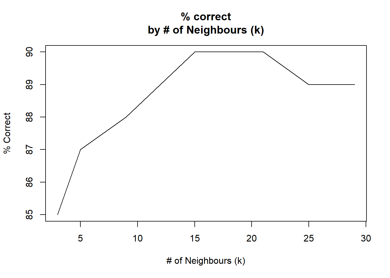
plot(kset, correct, type="h", main="% correct\nby # of Neighbours (k)",
     xlab="# of Neighbours (k)", ylab="% Correct")

# Using ggplot
library(ggplot2)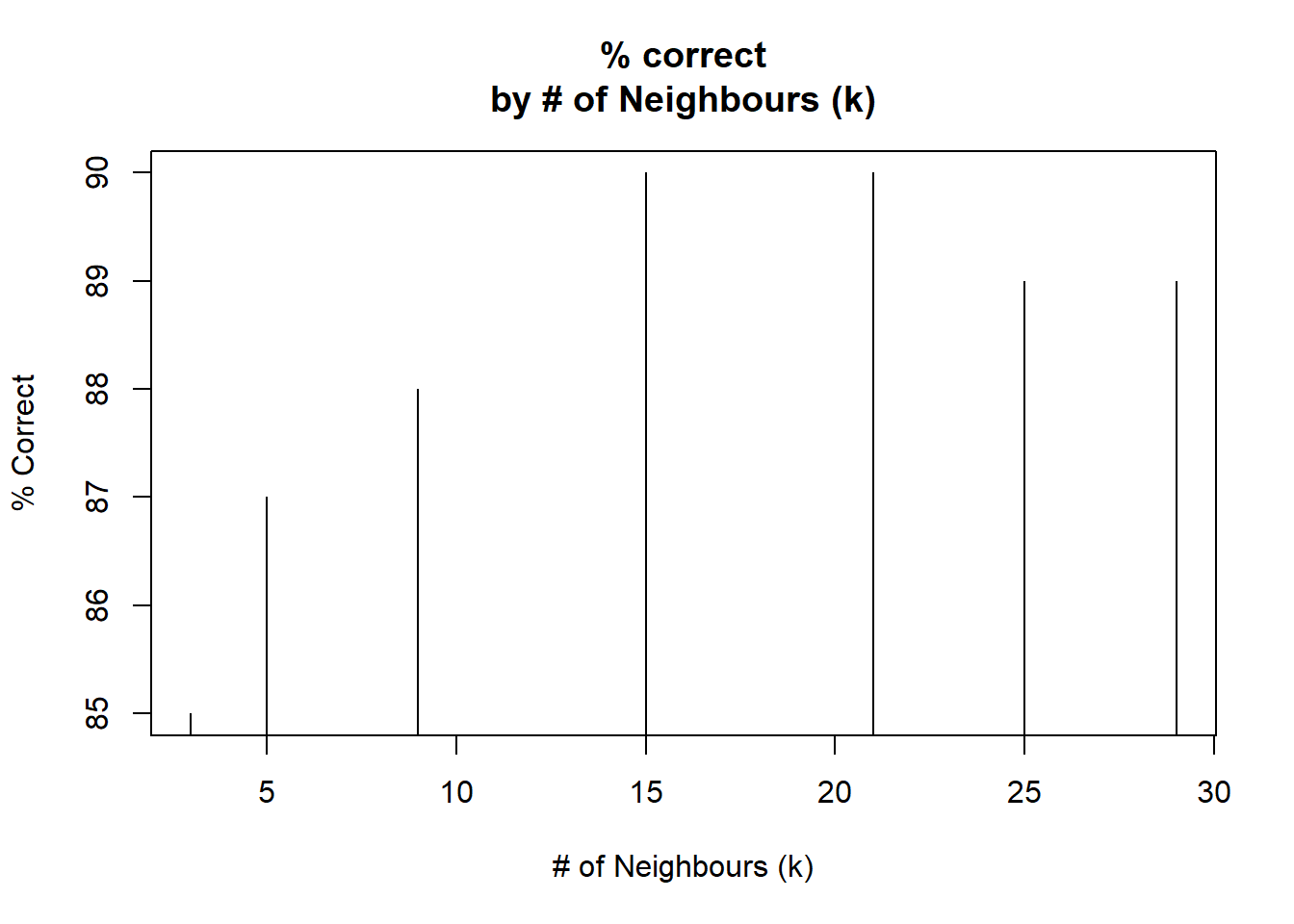
lc <- ggplot(data=k_opt, aes(x=kset, y=correct))
lc + geom_line() + geom_point() + xlab("# of Neighbours (k)") +
     ylab("% Correct") + ggtitle("% Correct Predictions\n- by k -")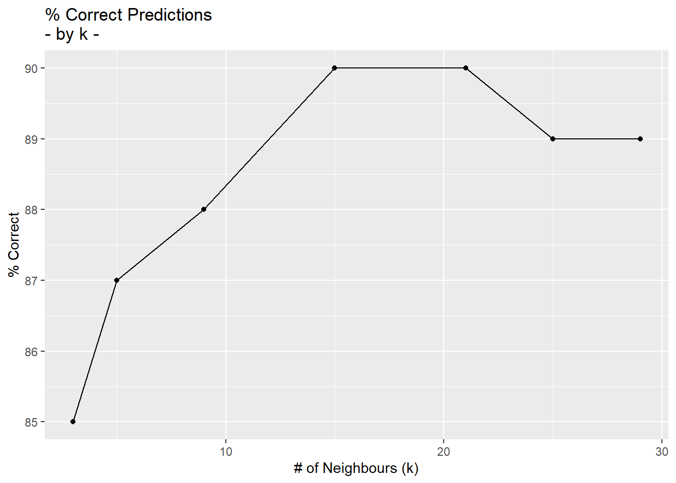
If we are satisfied with the model, a final step could be to make maximum use of all the information (all 500 records) in training the model, and then apply it to new applicants.