Chapter 6 Assignment: A Solution
6.1 kNN Method
The tasks and questions are:
- Read the file (cars.csv)
- Describe the file
- how many records?
- How many variables?
- What are the minimum, mean, and maximum values of those variables?
- Prepare the data before applying the kNN method.
- Determine the "label" variable!
- Normalize the file (excluding the "label" variable!). The resulting values of all variables should be in the range from 0 to 1.
- Create a training and test set. Use 80% of the records for the training set. The data may be sorted by important characteristics!
- Determine k.
- Train the model, and evaluate the model: how good are the predictions in the test set?
- What are possible improvements in the model? Apply it!
Tip: the data are on GitHub.
You can download the data, or read the data directly using:
cars <- read.csv("https://raw.githubusercontent.com/ssmresearch/hanminor/main/cars.csv")## KNN
rm(list=ls())
# Step 1: Read Data
cars <- read.csv("https://raw.githubusercontent.com/ssmresearch/hanminor/main/cars.csv")
head(cars)## origin price mileage repair headspace trunkspace weight length turningcircle
## 1 usa 4099 8.8 3 6.25 308 1318.5 465.0 12.20
## 2 usa 4749 6.8 3 7.50 308 1507.5 432.5 12.20
## 3 usa 3799 8.8 3 7.50 336 1188.0 420.0 10.68
## 4 usa 4816 8.0 3 11.25 448 1462.5 490.0 12.20
## 5 usa 7827 6.0 4 10.00 560 1836.0 555.0 13.12
## 6 usa 5788 7.2 3 10.00 588 1651.5 545.0 13.12
## gear_ratio
## 1 3.58
## 2 2.53
## 3 3.08
## 4 2.93
## 5 2.41
## 6 2.73str(cars)## 'data.frame': 74 obs. of 10 variables:
## $ origin : chr "usa" "usa" "usa" "usa" ...
## $ price : num 4099 4749 3799 4816 7827 ...
## $ mileage : num 8.8 6.8 8.8 8 6 7.2 10.4 8 6.4 7.6 ...
## $ repair : num 3 3 3 3 4 3 3 3 3 3 ...
## $ headspace : num 6.25 7.5 7.5 11.25 10 ...
## $ trunkspace : num 308 308 336 448 560 588 280 448 476 364 ...
## $ weight : num 1318 1508 1188 1462 1836 ...
## $ length : num 465 432 420 490 555 ...
## $ turningcircle: num 12.2 12.2 10.7 12.2 13.1 ...
## $ gear_ratio : num 3.58 2.53 3.08 2.93 2.41 2.73 2.87 2.93 2.93 3.08 ...# 10 variabels
# factor ("label") in first column
# "features" in kcolumns 2:10
# Step 2: Prepare Data
# 2.1 Normalize
normalizer <- function(x){
return((x-min(x))/(max(x)-min(x)))
}
# Normalize data (except the label)
cars_n <- as.data.frame(lapply(cars[,2:10], normalizer))
summary(cars_n) # check that values of all variables are between 0 and 1!## price mileage repair headspace
## Min. :0.00000 Min. :0.0000 Min. :0.000 Min. :0.0000
## 1st Qu.:0.07366 1st Qu.:0.2069 1st Qu.:0.500 1st Qu.:0.2857
## Median :0.13599 Median :0.2759 Median :0.500 Median :0.4286
## Mean :0.22784 Mean :0.3206 Mean :0.598 Mean :0.4266
## 3rd Qu.:0.24108 3rd Qu.:0.4397 3rd Qu.:0.750 3rd Qu.:0.5714
## Max. :1.00000 Max. :1.0000 Max. :1.000 Max. :1.0000
## trunkspace weight length turningcircle
## Min. :0.0000 Min. :0.0000 Min. :0.0000 Min. :0.0000
## 1st Qu.:0.2917 1st Qu.:0.1591 1st Qu.:0.3077 1st Qu.:0.2504
## Median :0.5000 Median :0.4643 Median :0.5549 Median :0.4501
## Mean :0.4865 Mean :0.4089 Mean :0.5048 Mean :0.4329
## 3rd Qu.:0.6528 3rd Qu.:0.5974 3rd Qu.:0.6786 3rd Qu.:0.6007
## Max. :1.0000 Max. :1.0000 Max. :1.0000 Max. :1.0000
## gear_ratio
## Min. :0.0000
## 1st Qu.:0.3176
## Median :0.4500
## Mean :0.4852
## 3rd Qu.:0.6838
## Max. :1.0000# 2.2 Training and test set
# Random sample of 80%
set.seed(98989) # For reproducible results
x <- nrow(cars_n) # bepaal aantal observeringen (74)
xs <- round(0.80*x,0)
cat("# of records:",x,"\nSample:", xs)## # of records: 74
## Sample: 59train_sample <- sample(x,xs) # sample xs out of x (approx 80%)
str(train_sample) # show the sample## int [1:59] 58 32 19 8 24 13 74 39 22 64 ...# split the data in training and test set (59 and 15 observations, respectively)
# For criteria, in columns 2:10, and for label variable (column 1)
cars_train <- cars_n[train_sample ,]
cars_test <- cars_n[-train_sample,]
cars_train_label <- cars[train_sample, 1]
cars_test_label <- cars[-train_sample, 1]
str(cars_train)## 'data.frame': 59 obs. of 9 variables:
## $ price : num 0.1417 0.0971 0.0526 0.1505 0.087 ...
## $ mileage : num 0.414 0.207 0.241 0.276 0.552 ...
## $ repair : num 0.75 0.5 0.5 0.5 0.75 0.5 1 0.5 0.25 0.75 ...
## $ headspace : num 0.286 0.429 0.571 0.143 0 ...
## $ trunkspace : num 0.167 0.556 0.444 0.611 0.222 ...
## $ weight : num 0.169 0.523 0.542 0.494 0.013 ...
## $ length : num 0.3077 0.6154 0.6044 0.6374 0.0549 ...
## $ turningcircle: num 0.151 0.501 0.601 0.55 0.101 ...
## $ gear_ratio : num 0.794 0.141 0.218 0.435 0.565 ...str(cars_test)## 'data.frame': 15 obs. of 9 variables:
## $ price : num 0.1156 0.0403 0.3596 0.1437 0.057 ...
## $ mileage : num 0.172 0.345 0.103 0.345 0.207 ...
## $ repair : num 0.5 0.5 0.75 0.25 0.25 0.5 0.75 0.75 0.5 0.5 ...
## $ headspace : num 0.429 0.429 0.714 0.143 0.714 ...
## $ trunkspace : num 0.333 0.389 0.833 0.611 0.667 ...
## $ weight : num 0.516 0.286 0.753 0.474 0.597 ...
## $ length : num 0.341 0.286 0.879 0.637 0.703 ...
## $ turningcircle: num 0.45 0.201 0.601 0.501 0.75 ...
## $ gear_ratio : num 0.2 0.524 0.129 0.318 0.165 ...str(cars_train_label); length(cars_train_label)## chr [1:59] "other" "usa" "usa" "usa" "usa" "usa" "other" "usa" "usa" ...## [1] 59str(cars_test_label) ; length(cars_test_label)## chr [1:15] "usa" "usa" "usa" "usa" "usa" "usa" "usa" "usa" "usa" "usa" ...## [1] 15# Step 3: Train model
# install.packages("class")
library(class)
# Choice of k: odd number
k <- round(sqrt(nrow(cars_n))) # Rule of thumb
cat("Rule of thumb, for k:",k)## Rule of thumb, for k: 9k <- ifelse(k%%2==0, k-1,k) # k is odd (9) already
cat("k is", k,"[ = odd number, approximate square root of",x,"]\n")## k is 9 [ = odd number, approximate square root of 74 ]cars_pred <- knn(train=cars_train, test=cars_test, cl=cars_train_label, k)
# Step 4: Evaluate Model
library(gmodels)
CrossTable(cars_test_label,cars_pred, expected=TRUE, format="SPSS")##
## Cell Contents
## |-------------------------|
## | Count |
## | Expected Values |
## | Chi-square contribution |
## | Row Percent |
## | Column Percent |
## | Total Percent |
## |-------------------------|
##
## Total Observations in Table: 15
##
## | cars_pred
## cars_test_label | other | usa | Row Total |
## ----------------|-----------|-----------|-----------|
## other | 3 | 0 | 3 |
## | 0.600 | 2.400 | |
## | 9.600 | 2.400 | |
## | 100.000% | 0.000% | 20.000% |
## | 100.000% | 0.000% | |
## | 20.000% | 0.000% | |
## ----------------|-----------|-----------|-----------|
## usa | 0 | 12 | 12 |
## | 2.400 | 9.600 | |
## | 2.400 | 0.600 | |
## | 0.000% | 100.000% | 80.000% |
## | 0.000% | 100.000% | |
## | 0.000% | 80.000% | |
## ----------------|-----------|-----------|-----------|
## Column Total | 3 | 12 | 15 |
## | 20.000% | 80.000% | |
## ----------------|-----------|-----------|-----------|
##
##
## Statistics for All Table Factors
##
##
## Pearson's Chi-squared test
## ------------------------------------------------------------
## Chi^2 = 15 d.f. = 1 p = 0.0001075112
##
## Pearson's Chi-squared test with Yates' continuity correction
## ------------------------------------------------------------
## Chi^2 = 9.401042 d.f. = 1 p = 0.002168622
##
##
## Minimum expected frequency: 0.6
## Cells with Expected Frequency < 5: 3 of 4 (75%)# Step 5: Improve Model
# Alternative values for k (3; 5; 7; 9; 11; 13; 15)
kset <- c(3, 5, 7, 9, 11, 13, 15)
(ssize <- x-xs) # opslaan van de steekproefomvang; 74 - 59 = 15## [1] 15for (k in kset) {
cars_pred <- knn(train=cars_train, test=cars_test,cl=cars_train_label,k)
true_neg <- table(cars_test_label,cars_pred)[1,1]
true_pos <- table(cars_test_label,cars_pred)[2,2]
corn = true_neg + true_pos
corp = 100*round((corn / ssize), 4)
cat("Correctly Predicted (k=", k,"):",corn, "(",corp,"%)\n")
}## Correctly Predicted (k= 3 ): 15 ( 100 %)
## Correctly Predicted (k= 5 ): 15 ( 100 %)
## Correctly Predicted (k= 7 ): 14 ( 93.33 %)
## Correctly Predicted (k= 9 ): 15 ( 100 %)
## Correctly Predicted (k= 11 ): 15 ( 100 %)
## Correctly Predicted (k= 13 ): 15 ( 100 %)
## Correctly Predicted (k= 15 ): 15 ( 100 %)correct <- c(15,15,14,15,15,15,15)
(k_opt <- data.frame(kset, correct))## kset correct
## 1 3 15
## 2 5 15
## 3 7 14
## 4 9 15
## 5 11 15
## 6 13 15
## 7 15 15plot(kset, correct, type="l", main="% correct\nby # of neighbours (k)",
xlab="# neighbours (k)", ylab="% Correct")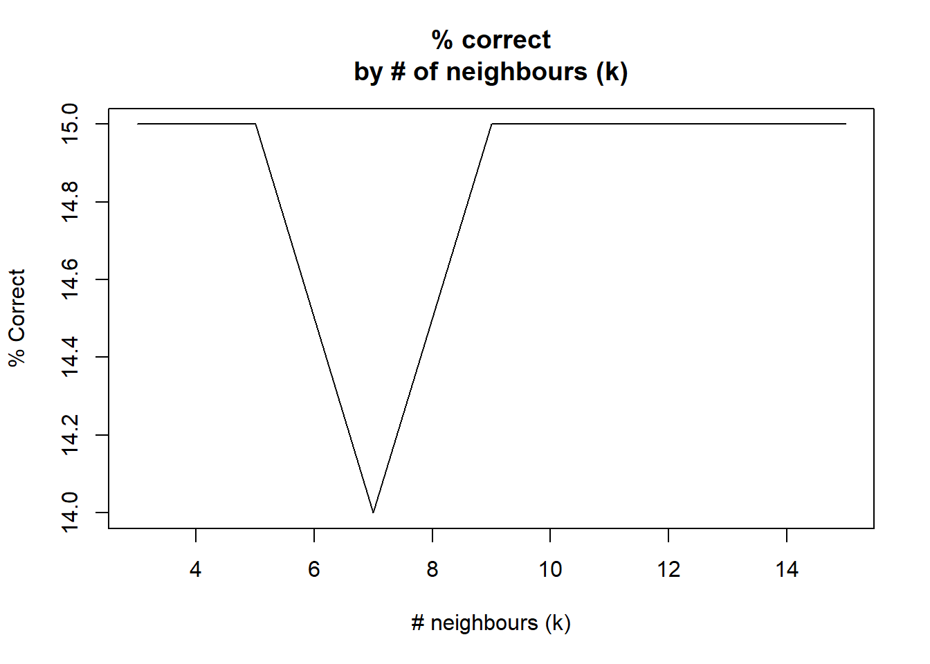
6.2 KMeans
## KMeans

rm(list=ls())
cars<-read.csv("cars.csv",header=TRUE)
str(cars)
## 'data.frame': 74 obs. of 10 variables:
## $ origin : chr "usa" "usa" "usa" "usa" ...
## $ price : num 4099 4749 3799 4816 7827 ...
## $ mileage : num 8.8 6.8 8.8 8 6 7.2 10.4 8 6.4 7.6 ...
## $ repair : num 3 3 3 3 4 3 3 3 3 3 ...
## $ headspace : num 6.25 7.5 7.5 11.25 10 ...
## $ trunkspace : num 308 308 336 448 560 588 280 448 476 364 ...
## $ weight : num 1318 1508 1188 1462 1836 ...
## $ length : num 465 432 420 490 555 ...
## $ turningcircle: num 12.2 12.2 10.7 12.2 13.1 ...
## $ gear_ratio : num 3.58 2.53 3.08 2.93 2.41 2.73 2.87 2.93 2.93 3.08 ...# normaliseren van data
normalizer <- function(x){
return((x-min(x))/(max(x)-min(x)))
}
# Include origin (now a factor variable; redefine as dummy 0/1)
cars2 <- cars # copy of cars
# Add dummy for origin
cars2$originDum <- ifelse(cars2$origin=="usa",1,0)
str(cars2)## 'data.frame': 74 obs. of 11 variables:
## $ origin : chr "usa" "usa" "usa" "usa" ...
## $ price : num 4099 4749 3799 4816 7827 ...
## $ mileage : num 8.8 6.8 8.8 8 6 7.2 10.4 8 6.4 7.6 ...
## $ repair : num 3 3 3 3 4 3 3 3 3 3 ...
## $ headspace : num 6.25 7.5 7.5 11.25 10 ...
## $ trunkspace : num 308 308 336 448 560 588 280 448 476 364 ...
## $ weight : num 1318 1508 1188 1462 1836 ...
## $ length : num 465 432 420 490 555 ...
## $ turningcircle: num 12.2 12.2 10.7 12.2 13.1 ...
## $ gear_ratio : num 3.58 2.53 3.08 2.93 2.41 2.73 2.87 2.93 2.93 3.08 ...
## $ originDum : num 1 1 1 1 1 1 1 1 1 1 ...table(cars2$origin,cars2$originDum)##
## 0 1
## other 22 0
## usa 0 52cars2$origin<-NULL
# normalize
cars2_n <- as.data.frame(lapply(cars2, normalizer))
summary(cars2_n)## price mileage repair headspace
## Min. :0.00000 Min. :0.0000 Min. :0.000 Min. :0.0000
## 1st Qu.:0.07366 1st Qu.:0.2069 1st Qu.:0.500 1st Qu.:0.2857
## Median :0.13599 Median :0.2759 Median :0.500 Median :0.4286
## Mean :0.22784 Mean :0.3206 Mean :0.598 Mean :0.4266
## 3rd Qu.:0.24108 3rd Qu.:0.4397 3rd Qu.:0.750 3rd Qu.:0.5714
## Max. :1.00000 Max. :1.0000 Max. :1.000 Max. :1.0000
## trunkspace weight length turningcircle
## Min. :0.0000 Min. :0.0000 Min. :0.0000 Min. :0.0000
## 1st Qu.:0.2917 1st Qu.:0.1591 1st Qu.:0.3077 1st Qu.:0.2504
## Median :0.5000 Median :0.4643 Median :0.5549 Median :0.4501
## Mean :0.4865 Mean :0.4089 Mean :0.5048 Mean :0.4329
## 3rd Qu.:0.6528 3rd Qu.:0.5974 3rd Qu.:0.6786 3rd Qu.:0.6007
## Max. :1.0000 Max. :1.0000 Max. :1.0000 Max. :1.0000
## gear_ratio originDum
## Min. :0.0000 Min. :0.0000
## 1st Qu.:0.3176 1st Qu.:0.0000
## Median :0.4500 Median :1.0000
## Mean :0.4852 Mean :0.7027
## 3rd Qu.:0.6838 3rd Qu.:1.0000
## Max. :1.0000 Max. :1.0000# optimal number of clusters
c <- 10 # max number for wss-plot
wss <- (nrow(cars2_n)-1)*sum(apply(cars2_n,2,var)); wss[1]## [1] 52.77075for (i in 2:c) wss[i] <- sum(kmeans(cars2_n, centers=i)$withinss)
plot(1:c, wss, type="b", xlab="# of Clusters", ylab="Heterogeneity")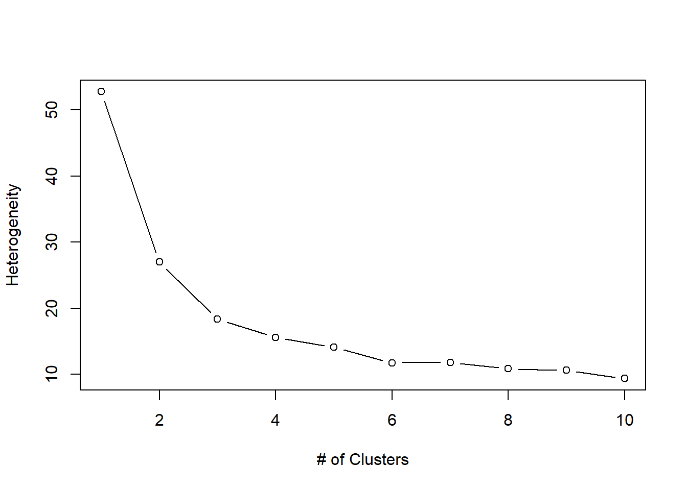
# Elbow at 3. Agree?

library(stats)
set.seed(111)
autoCluster <- kmeans(cars2_n, 3)
autoCluster$size
## [1] 30 22 22round(autoCluster$centers, 2)## price mileage repair headspace trunkspace weight length turningcircle
## 1 0.31 0.17 0.52 0.64 0.68 0.65 0.74 0.63
## 2 0.10 0.40 0.49 0.24 0.35 0.31 0.40 0.37
## 3 0.25 0.44 0.82 0.32 0.36 0.18 0.29 0.22
## gear_ratio originDum
## 1 0.28 1
## 2 0.47 1
## 3 0.77 0# Add cluster (1, 2 of 3) to data set
cars2$cluster <- autoCluster$cluster
# Aggregate (or summarize) info
names(cars2)## [1] "price" "mileage" "repair" "headspace"
## [5] "trunkspace" "weight" "length" "turningcircle"
## [9] "gear_ratio" "originDum" "cluster"aggregate(data=cars2, mileage ~ cluster, mean)## cluster mileage
## 1 1 6.786667
## 2 2 9.490909
## 3 3 9.909091aggregate(data=cars2, length ~ cluster, mean)## cluster length
## 1 1 523.2500
## 2 2 445.4545
## 3 3 421.3636aggregate(data=cars2, price ~ cluster, mean)## cluster price
## 1 1 7225.967
## 2 2 4499.409
## 3 3 6384.682aggregate(data=cars2, price ~ cluster, min)## cluster price
## 1 1 3291
## 2 2 3299
## 3 3 3748aggregate(data=cars2, price ~ cluster, max)## cluster price
## 1 1 15906
## 2 2 6486
## 3 3 12990# install.packages("doBy")
library(doBy)## Warning: package 'doBy' was built under R version 4.0.4summaryBy(list(c("price","headspace","originDum"), c("cluster")), data=cars2, FUN=c(min,mean,max))## cluster price.min headspace.min originDum.min price.mean headspace.mean
## 1 1 3291 6.25 1 7225.967 9.375000
## 2 2 3299 3.75 1 4499.409 5.852273
## 3 3 3748 3.75 0 6384.682 6.534091
## originDum.mean price.max headspace.max originDum.max
## 1 1 15906 12.50 1
## 2 1 6486 10.00 1
## 3 0 12990 8.75 0