Chapter 1 Monarchy or Republic?
1.1 Dataset
library(dplyr)
R19460602 <- read.csv("data/R19460602.txt", sep = ";")

# Remove non informative columns
R19460602 <- R19460602 %>%
  Filter(function(x) any(x != 0), .) %>%
  select(-c(4, 5))

R19460602 <- R19460602 %>%
  rename(MONARCHIA = NUMVOTINO, REPUBBLICA = NUMVOTISI) %>%
  mutate(across(c(VOTANTI, ELETTORI, REPUBBLICA, MONARCHIA, SCHEDE_BIANCHE), as.numeric)) %>%
  mutate(across(c(PROVINCIA, COMUNE), factor)) %>%
  mutate(
    SCHEDE_NON_VALIDE = VOTANTI - (REPUBBLICA + MONARCHIA),
    REPUBBLICA_PERC = (REPUBBLICA / (VOTANTI - SCHEDE_NON_VALIDE)) * 100,
    MONARCHIA_PERC = (MONARCHIA / (VOTANTI - SCHEDE_NON_VALIDE)) * 100,
    AFFLUENZA = (VOTANTI / ELETTORI) * 100
  )


DT::datatable(R19460602, filter = "top", options = list(
  scrollX = TRUE, autowidth = TRUE
))library(tidyr)
library(dplyr)
library(ggplot2)
# Prepare data for pie chart
summary_abs <- R19460602 %>%
summarise(
Monarchy = sum(MONARCHIA),
Republic = sum(REPUBBLICA)
) %>%
pivot_longer(
cols = everything(),
names_to = "Forma",
values_to = "Voti"
) %>%
mutate(
Perc = (Voti / sum(Voti)) * 100,
Text = paste0(round(Perc, 2), "%") # Percentage text label for the pie chart
)
# Pie chart
ggplot(summary_abs, aes(x = "", y = Voti, fill = Forma)) +
geom_bar(stat = "identity", width = 1) + # Create bar chart (base for the pie)
coord_polar("y") + # Transform bar chart into a pie chart
geom_text(aes(label = Text), color = "white", size = 5,
position = position_stack(vjust = 0.5)) + # Add percentage labels
scale_fill_manual(values = c("Monarchy" = "red", "Republic" = "blue")) +
theme_void() +
theme(legend.title = element_blank(),
plot.title = element_text(size = 16, face = "bold", hjust = 0.5)) #+ # Center the title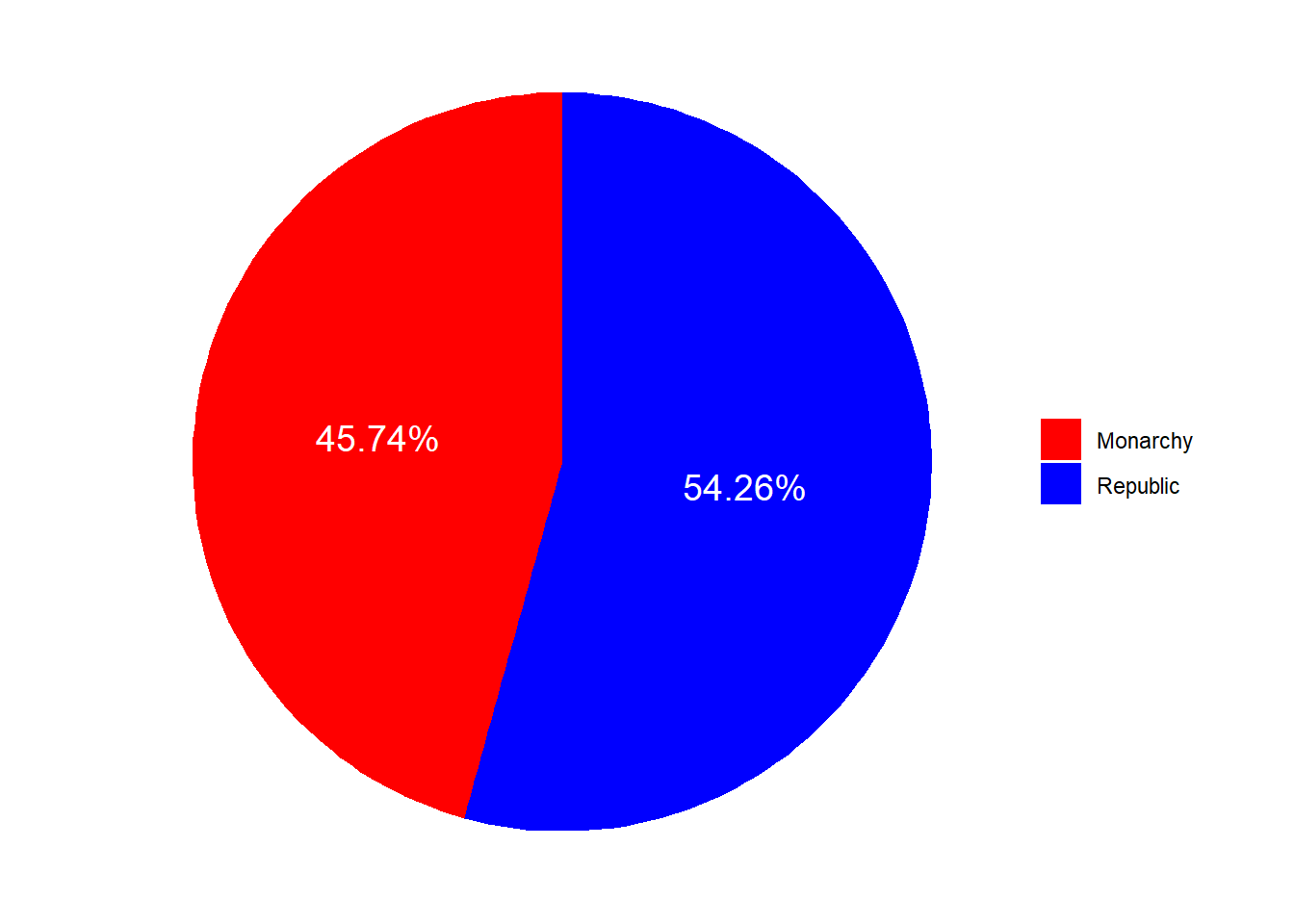
Figure 1.1: Results of the 1946 Referendum. A pie chart was chosen because we are dealing with proportions and only two categories (Monarchy and Republic). Pie charts are ideal for displaying simple fractions, making it easy to highlight that the Republic won by a narrow margin. Percentages are added as labels to provide exact values. The associated colors (blue for the Republic and red for the Monarchy) ensure consistency throughout the chapter, helping viewers easily interpret the results. Thus, legend is omitted for the subsequent graphs
library(sf)
shape_data <- st_read("C:\\Users\\acer\\Desktop\\electoral_differences_regions\\Province_1951", options = "ENCODING=UTF-8")
## options: ENCODING=UTF-8
## Reading layer `Province_1951' from data source
## `C:\Users\acer\Desktop\electoral_differences_regions\Province_1951' using driver `ESRI Shapefile'
## Simple feature collection with 92 features and 2 fields
## Geometry type: MULTIPOLYGON
## Dimension: XY
## Bounding box: xmin: 313361 ymin: 3933879 xmax: 1312107 ymax: 5220491
## Projected CRS: ED50 / UTM zone 32N# Calculate the centroide (geographic center) of each province
shape_data <- shape_data %>%
mutate(centroid = st_centroid(geometry)) %>% # Compute the centroid of each geometry
mutate(lat = st_coordinates(centroid)[,2]) # Extract latitude coordinate from the centroid
# Group and summarize the election data by PROVINCIA and CIRCOSCRIZIONE
dati_raggruppati <- R19460602 %>%
group_by(PROVINCIA, CIRCOSCRIZIONE) %>%
summarize(
TOTAL_ELETTORI = sum(ELETTORI, na.rm = TRUE),
TOTAL_VOTANTI = sum(VOTANTI, na.rm = TRUE),
TOTAL_REPUBBLICA = sum(REPUBBLICA, na.rm = TRUE),
TOTAL_MONARCHIA = sum(MONARCHIA, na.rm = TRUE),
SCHEDE_BIANCHE = sum(SCHEDE_BIANCHE, na.rm = TRUE),
SCHEDE_NON_VALIDE = sum(SCHEDE_NON_VALIDE, na.rm = TRUE),
AFFLUENZA_MEDIA = mean(AFFLUENZA, na.rm = TRUE)
) %>%
mutate(TOTAL_PERC_REPUBBLICA = (TOTAL_REPUBBLICA/(TOTAL_MONARCHIA+TOTAL_REPUBBLICA))*100)
# Order the provinces by their latitude
province_ordinate <- shape_data %>%
arrange(desc(lat)) %>%
select(DEN_PROV, lat) %>%
rename(PROVINCIA = DEN_PROV)
#check for PROVINCE names not properly encoded in UTF-8
invalid_entries <- province_ordinate[!iconv(province_ordinate$PROVINCIA, "UTF-8", "UTF-8", sub = "byte") == province_ordinate$PROVINCIA, ]
#View(invalid_entries) # Forlì
province_ordinate$PROVINCIA[40] <- "Forli'"
# Standardize the province names (lowercase and remove extra whitespace)
province_ordinate <- province_ordinate %>%
mutate(PROVINCIA = tolower(trimws(PROVINCIA)))
dati_raggruppati <- dati_raggruppati %>%
mutate(PROVINCIA = tolower(trimws(PROVINCIA)))
# Identify missing provinces (provinces in shape data but not in election data)
province_mancanti <- province_ordinate %>%
anti_join(dati_raggruppati, by = "PROVINCIA")
#province_mancanti$PROVINCIA
# [1] "bolzano - bozen" "gorizia" "trieste"
# [4] "valle d'aosta" "reggio nell'emilia" "massa-carrara"
# [7] "pesaro urbino" "reggio di calabria"
#shape file is from 1951 (it was the oldest one available) so bolzano - bozen, gorizia e trieste are missing because they were not yet part of Italy in 1946
# Define a dictionary of substitutions to standardize the remeaning province names
sostituzioni <- c(
"valle d'aosta" = "aosta",
"reggio nell'emilia" = "reggio emilia",
"massa-carrara" = "massa carrara",
"pesaro urbino" = "pesaro",
"reggio di calabria" = "reggio calabria"
)
# Apply the substitutions to both datasets
dati_raggruppati <- dati_raggruppati %>%
mutate(PROVINCIA = recode(PROVINCIA, !!!sostituzioni))
province_ordinate <- province_ordinate %>%
mutate(PROVINCIA = recode(PROVINCIA, !!!sostituzioni))
# Join the two datasets by PROVINCIA to merge election data with geographic information
dati_completi <- province_ordinate %>%
left_join(dati_raggruppati, by = "PROVINCIA")
#Create a new column with formatted text for display in the plot
dati_completi <- dati_completi %>%
mutate(Inter = paste0(PROVINCIA, ": ", round(TOTAL_PERC_REPUBBLICA, 2), "%")) #
# library(scales)
# grafico <- ggplot(data = dati_completi) +
# geom_sf(aes(geometry = geometry, fill = TOTAL_PERC_REPUBBLICA),
# color = "white") +
# scale_fill_gradientn(colours = c("white", "darkblue"),
# values = scales::rescale(c(0, 25, 50, 75)),
# na.value = "white",
# name = "Voti Repubblica",
# labels = percent_format(scale = 1)) +
# labs(title = "Referendum 1946") +
# theme_void() +
# theme(
# plot.title = element_text(hjust = 0.5),
# legend.position = "right"
# )
# graficolibrary(stringr)
#uniform capitalization
dati_completi_regione <- dati_completi %>%
mutate(PROVINCIA = str_to_title(PROVINCIA, locale = "it")) #ex. napoli -> Napoli
province_ordinate <- province_ordinate %>%
mutate(PROVINCIA = str_to_title(PROVINCIA, locale = "it"))
#dictionary mapping each region (key) to its provinces (values)
Region_dict <- list(
"Piemonte" = c("Torino", "Vercelli", "Novara", "Cuneo", "Asti", "Alessandria", "Biella", "Verbano-Cusio-Ossola"),
"Valle d'Aosta/Vallée d'Aoste" = c("Aosta"),
"Liguria" = c("Imperia", "Savona", "Genova", "La Spezia"),
"Lombardia" = c("Varese", "Como", "Sondrio", "Milano", "Bergamo", "Brescia", "Pavia", "Cremona", "Mantova", "Lecco", "Lodi", "Monza e della Brianza"),
"Trentino-Alto Adige/Südtirol" = c("Bolzano - Bozen", "Trento"),
"Veneto" = c("Verona", "Vicenza", "Belluno", "Treviso", "Venezia", "Padova", "Rovigo"),
"Friuli-Venezia Giulia" = c("Udine", "Gorizia", "Trieste", "Pordenone"),
"Emilia-Romagna" = c("Piacenza", "Parma", "Reggio Emilia", "Modena", "Bologna", "Ferrara", "Ravenna", "Forli'", "Rimini"),
"Toscana" = c("Massa Carrara", "Lucca", "Pistoia", "Firenze", "Livorno", "Pisa", "Arezzo", "Siena", "Grosseto", "Prato"),
"Umbria" = c("Perugia", "Terni"),
"Marche" = c("Pesaro", "Ancona", "Macerata", "Ascoli Piceno", "Fermo"),
"Lazio" = c("Viterbo", "Rieti", "Roma", "Latina", "Frosinone"),
"Abruzzo" = c("L'aquila", "Teramo", "Pescara", "Chieti"),
"Molise" = c("Campobasso", "Isernia"),
"Campania" = c("Caserta", "Benevento", "Napoli", "Avellino", "Salerno"),
"Puglia" = c("Foggia", "Bari", "Taranto", "Brindisi", "Lecce", "Barletta-Andria-Trani"),
"Basilicata" = c("Potenza", "Matera"),
"Calabria" = c("Cosenza", "Catanzaro", "Reggio Calabria", "Crotone", "Vibo Valentia"),
"Sicilia" = c("Trapani", "Palermo", "Messina", "Agrigento", "Caltanissetta", "Enna", "Catania", "Ragusa", "Siracusa"),
"Sardegna" = c("Sassari", "Nuoro", "Cagliari", "Oristano", "Sud Sardegna")
)
get_region <- function(provincia) {
for (region in names(Region_dict)) {
if (provincia %in% Region_dict[[region]]) {
return(region)
}
}
return(NA)
}
#associate each PROVINCIA to its region
dati_completi_regione$REGIONE <- sapply(dati_completi_regione$PROVINCIA, get_region)
#dati_completi[is.na(dati_completi$REGIONE), ]$PROVINCIAlibrary(ggplot2)
library(dplyr)
library(ggmosaic)
library(plotly)
north_regions <- c("Trentino-Alto Adige/Südtirol", "Friuli-Venezia Giulia", "Lombardia", "Veneto", "Piemonte", "Liguria", "Valle d'Aosta/Vallée d'Aoste", "Emilia-Romagna", "Toscana", "Marche", "Umbria")
south_regions <- c("Campania", "Calabria", "Sicilia", "Puglia", "Abruzzo", "Molise", "Sardegna", "Basilicata", "Lazio")
# Add a new column indicating if the region is in the North or South
# Summarize the data to get the total votes for Monarchia and Repubblica for each North/South region
mosaic_data <- dati_completi_regione %>%
mutate(North_South = case_when(
REGIONE %in% north_regions ~ "North",
REGIONE %in% south_regions ~ "South"
)) %>%
group_by(North_South) %>%
summarise(
TOTAL_REPUBBLICA = sum(TOTAL_REPUBBLICA, na.rm = TRUE),
TOTAL_MONARCHIA = sum(TOTAL_MONARCHIA, na.rm = TRUE)
) %>%
ungroup() %>% sf::st_drop_geometry()
#need for a long format for the mosaic
mosaic_data <- data.frame(
North_South = rep(c("North", "South"), each = 2),
Forma = rep(c("Monarchy", "Republic"), 2),
Voti = c(4780664, 9348858, 5936872, 3367520)
)
# Make the mosaic plot
mosaic <- ggplot(mosaic_data) +
geom_mosaic(aes(weight = Voti, x = product(North_South), fill = Forma)) +
scale_fill_manual(values = c("Republic" = "blue", "Monarchy" = "red")) +
theme_minimal() +
labs(title = "",
x = "",
y = "") +
theme(legend.position = "none", legend.title = element_blank()) +
theme_mosaic()
ggplotly(mosaic) %>% layout(showlegend = FALSE) #plotly ignora legend.position = "none"!!Figure 1.2: Results in North and South. Here, proportions are specified according to 2 categorical variables so a mosaic plot is used. We see that results were very different in North and South.
# contingency table
table_data <- xtabs(Voti ~ North_South + Forma, data = mosaic_data)
chi_test <- chisq.test(table_data)
chi_test
##
## Pearson's Chi-squared test with Yates' continuity correction
##
## data: table_data
## X-squared = 2030725, df = 1, p-value < 2.2e-16dati_regione <- dati_completi_regione %>%
group_by(REGIONE) %>%
summarize(PERC_REPUBBLICA = mean(TOTAL_PERC_REPUBBLICA, na.rm = TRUE), ELETTORI=sum(TOTAL_ELETTORI, na.rm=T), VOTANTI=sum(TOTAL_VOTANTI, na.rm=T)) %>%
mutate(WINNER = if_else(PERC_REPUBBLICA > 50, "Repubblica", "Monarchia")) %>%
mutate(WINNER = factor(WINNER, levels = c("Repubblica", "Monarchia")))
ggplot(data = dati_regione) +
geom_sf(aes(geometry = geometry, fill = WINNER),
color = "white") +
# coord_sf(expand = FALSE)+
scale_fill_manual(values = c("Repubblica" = "blue", "Monarchia" = "red"),
name = "Vincitore",
na.value = "white",
labels = c("Repubblica", "Monarchia")) +
#labs(title = "Referendum 1946", subtitle= "Who won in each region?") +
theme_void() +
theme(
plot.title = element_text(hjust = 0, size = 16),
legend.position = "none"
)
Figure 1.3: Choroplet map by region. Each region is colored based on the istitutional form which prevailed. Such a map shows clearly the divide between North and South. In all soutehrn regions Monarchy won, while in all northern ones Republic prevailed.
library(cartogram)
#adjust size of regions based on number of ELETTORI
cartogram_data <- cartogram_cont(dati_regione, weight = "ELETTORI")

ggplot(data = cartogram_data) +
  geom_sf(aes(geometry = geometry, fill = WINNER),
          color = "white") +
  coord_sf(expand = FALSE) +
  scale_fill_manual(values = c("Repubblica" = "blue", "Monarchia" = "red"),
                    name = "Vincitore",
                    na.value = "white",
                    labels = c("Repubblica", "Monarchia")) +
  #labs(title = "Referendum 1946", subtitle = "Who won in each region?") +
  theme_void() +
  theme(
    plot.title = element_text(size = 16, hjust=0),
    legend.position = "none"
  )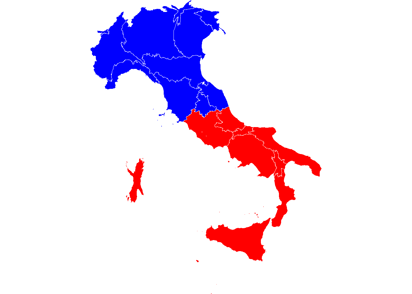
Figure 1.4: Cartogram map by region. Here the size of each region reflects the number of eligible voters. It highlights that regions, such as Sardinia, contributed less to the final result because of the few number of voters. Other regions like Lombardia are insted bigger in the cartogram.
library(plotly)
#take only relevant columns
dati_regione_dumbell <- sf::st_drop_geometry(dati_regione)[, c("PERC_REPUBBLICA","REGIONE")]

#order by percentage of votes for REPUBBLICA (ascending order)
dati_regione_dumbell <- dati_regione_dumbell[order(dati_regione_dumbell$PERC_REPUBBLICA), ]

dumbell_interactive <- plot_ly(dati_regione_dumbell) %>%
  add_segments(
    x = ~PERC_REPUBBLICA, y = ~REGIONE,
    xend = ~(100-PERC_REPUBBLICA), yend = ~REGIONE,
    color = I("grey"), showlegend = FALSE
  ) %>%
  add_markers(
    x = ~(100-PERC_REPUBBLICA), y = ~REGIONE,
    color = I("red"),
    name = "Monarchia"
  ) %>%
  add_markers(
    x = ~PERC_REPUBBLICA, y = ~REGIONE,
    color = I("blue"),
    name = "Repubblica"
  ) %>%
  layout(
    xaxis = list(title = "Percentage"),
    yaxis = list(
      title = "Region",
      categoryorder = "array",
      categoryarray = dati_regione_dumbell$REGIONE
    )
  )
dumbell_interactive
Figure 1.5: Percentage by regions. Percentage for Monarchy and Republic is shown. A dumbell plot has been chosen instead of bars because in this way the focus is on the points, corresponding to the percentage. With bars instead differences in percentages would have been less evident, with the eye drawn to the middle of the bars instead to their endpoints. Regions are ordered accoridng to the percentage for Repubblica, in descending order.
#compute winner in each province
dati_completi_province <- dati_completi %>%
  mutate(WINNER = factor(if_else(TOTAL_PERC_REPUBBLICA > 50, "Repubblica", "Monarchia"),
                         levels = c("Repubblica", "Monarchia")))

choroplet_province_winner <- ggplot(data = dati_completi_province) +
  geom_sf(aes(geometry = geometry, fill = WINNER),
          color = "white") +
  scale_fill_manual(values = c("Repubblica" = "blue", "Monarchia" = "red"),
                    na.value = "white",
                    name = "Vincitore",
                    labels = c("Repubblica", "Monarchia")) +
  #labs(title = "Referendum 1946", subtitle = "Who won in each province?") +
  theme_void() +
  theme(
    plot.title = element_text(hjust = 0),
    legend.position = "none"
  )

print(choroplet_province_winner)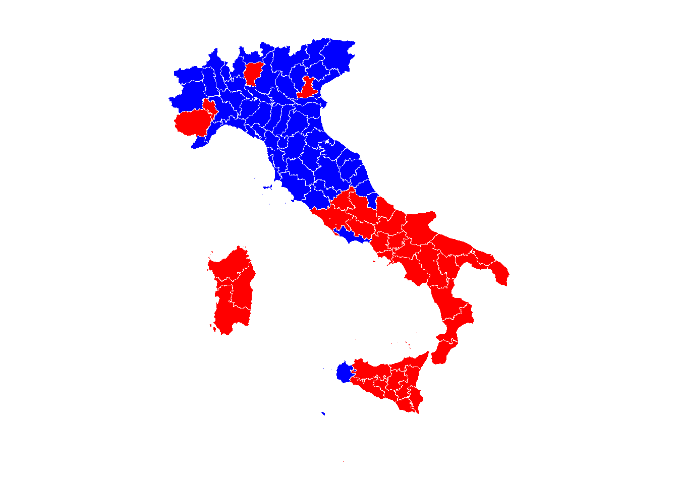
Figure 1.6: Choroplet map by provinces. Here data are shown at a higher level of granularity. It’s still clear the division North/South. few provinces deviated from their region’s overall outcome. Specifically: Cuneo and Asti in Piemonte, Bergamo in Lombardia, Latina in Lazio, Trapani in Sicilia. Note that Gorizia and Trieste were not yet part of Italy in 1946 so are not shown. This explains also why Friuly Venezia Giulia is so small in the previous cartogram