Chapter 6 Hypothesis Testing

6.1 Motivation
It’s time to formalize one of the major introductory inference topics. Much of this book has been focused on quantifying uncertainty around unknown parameters: Hypothesis Testing provides a new and powerful way to make claims about underlying parameters.
6.2 Introduction to Hypothesis Testing
Much like a lot of inference to this point, Hypothesis Testing asks you to think in a slightly different way for a naturally intuitive and probably familiar topic. Hopefully by now you are comfortable with the basics of this concept (either from introductory statistics or the introduction to this book), but in case you need a refresher this will get you up to speed.
Most of this book has tried to make claims about some unknown parameter, usually denoted \(\theta\), like the true average foot size of college males (this ‘parameter’ could be a single parameter or a set of parameters). We’ve learned how to build confidence intervals (Frequentist approach) and credible intervals (Bayesian approach) for these unknown quantities. Hypothesis testing is a little bit more direct, since it allows you to test a parameter being in a certain interval or value of your choosing.
First, let’s give the mathematical background. Say that some parameter \(\theta\) that you are interested in lies in the set \(\Omega\). You can think of \(\Omega\) kind of like the support of \(\theta\); it just gives all the possible values that \(\theta\) could take on (for example, if \(\theta\) is the true probability of it being rainy on a random day in Boston, then \(\Omega\) is the interval 0 to 1, since these are the bounds for a probability). Now envision two subsets of \(\Omega\), called \(\Omega_0\) and \(\Omega_1\), that partition \(\Omega\) (remember, partition means that they are disjoint and cover the entire space: for example, the sets \(\{1,2\}\) and \(\{3,4,5\}\) partition the set \(\{1,2,3,4,5\}\)). By construction, we know that \(\theta\) is either in \(\Omega_0\) or \(\Omega_1\) (from the last example, if \(\theta\) is a single value in the set \(\{1,2,3,4,5\}\), then it’s either in the set \(\{1,2\}\) or \(\{3,4,5\}\) but not both). From here, we generate our hypothesis: the Null Hypothesis, or \(H_0\), states that \(\theta\) is in \(\Omega_0\), and the Alternative Hypothesis states that \(\theta\) is in \(\Omega_1\).
Let’s ground this a little bit. Say, from before, that we are interested in the parameter \(p\) that gives the true probability of rain on a random day. In this case, we know that \(\Omega\), the set that contains all possible values for \(p\), is just the interval \([0,1]\) because we are working with a probability (which must be from 0 and 1). Say you are pretty sure that it rains less than half the time, but want to test if it rains half or more of the time. In this case, the two subsets that partition \(\Omega\) are \([0,.5)\) and \([.5,1]\) where the ‘\([\)’ means inclusive - the interval contains the endpoint - and ‘(’ means exclusive - the interval does not contain the endpoint. Your null hypothesis is that \(p\) is in the interval \([0,.5)\) and your alternative hypothesis is that \(p\) is in the interval \([.5,1]\). This corresponds to:
\[H_0: p < .5, \; \; H_A: p \geq .5\]
If you got enough evidence that indicated \(p < .5\), you would fail to reject the null hypothesis. Remember you can never fully reject the null hypothesis, since we can’t actually collect all the data and find the true parameter. If there was enough evidence that indicated \(p \geq .5\), you would reject the null hypothesis in favor of the alternative hypothesis. We’ll formalize what ‘enough evidence’ means in later parts.
6.3 Permutations of Hypothesis Testing
Hypothesis Tests come in all shapes and sizes. Here are the major forms you will likely see.
1. Simple vs. Composite Hypothesis
A simple hypothesis consists of one potential value for the parameter \(\theta\). For example, a simple hypothesis might be \(H_0: p = .5\) or \(H_A: \bar{X} = 7.6\). A composite hypothesis has a whole range of values for the parameter. For example, \(H_0: p < .6\), or \(H_A: \bar{X} \geq 5.4\). It’s important to remember that null and alternative hypotheses can be both simple and composite.
2. One-sided vs. Two-sided
For a one-sided test, both hypotheses are composite; that is, the null covers one range, and the alternative covers another range. The example we did earlier is one-sided:
\[H_0: p < .5, \; \; H_A: p \geq .5\]
For a two-sided test, the null hypothesis is simple (that is, fixes on one value) and the alternative is composite so that it covers the rest of the sample space. We could tweak the above to make it two-sided:
\[H_0: p = .4, \; \; H_A: p \neq .4\]
Notice how in both cases, both Hypotheses cover the entire sample space. Technically, that’s because \(\Omega_0\) and \(\Omega_1\), the null and alternative sets that may contain \(\theta\), partition the entire space \(\theta\).
6.4 Testing Structure
Now we’ll talk about the actual mechanics of testing. It’s best to learn these in a more general sense so you can be more flexible in your application, as opposed to the plug-and-chug recipe that introductory statistics provides.
To actually test something, you need a test statistic. This is just a function of your data (i.e., one function would simply be the mean of your data). You reject your null hypothesis if this test statistic falls in the ‘rejection region’ (a predetermined region; we will talk more about this soon).
For example, let’s say you wanted to test if the average weight of college males was over 150, and you set up the following Hypotheses, where \(\mu\) is the true average weight.
\[H_0: \mu \leq 150, \; \; H_A: \mu > 150\]
This is a one-sided test where both Hypotheses are composite.
A natural test statistic would be \(\bar{X}\), the sample mean. We say this is ‘natural’ because it’s intuitive; if you want to test what the true mean of a population would be, wouldn’t you think to look at the sample mean? Now, let’s decide on our rejection region. It seems reasonable that you will reject the null hypothesis (that is, you conclude that the average mean is over 150) if the sample mean was over 165, since it’s a good deal higher than 150. Yes, this is an arbitrary cutoff; we’ll formalize how we choose the region later, this is just for intuition. So, in this case, we would collect our test statistic, which is just the mean of our sample, and see if it falls in our rejection region. If the sample mean is greater than 165, we reject the null hypothesis and say there’s sufficient evidence that the average college height is greater than 165.
Makes sense. Now, let’s push a bit more and talk about errors; specifically, Type I and Type II Errors. These have pretty straightforward definitions:
- Type I Error: rejecting a true null hypothesis
- Type II Error: failing to reject a false null hypothesis
These are intuitive because there are two potential outcomes for the null hypothesis (either it is true or not) and we have two potential choices (reject it or not) for 4 total permutations. Two of those permutations are correct: when we reject a false null, or fail to reject a true null, and then the other two are incorrect (and defined in terms of error here).
You can think of these in a courtroom setting: a Type I Error is sentencing (rejecting) an innocent person (a true null hypothesis, since everyone is innocent until proven guilty), and a Type II Error is letting go (failing to reject) a guilty person (a false null hypothesis). Generally, Type I Errors are more serious, so we first try to minimize those. As you will see, when you try to minimize one error, you usually have a higher chance of getting the other. For example, what’s the only way you could guarantee never getting a Type I error? Well, you would have to never reject the null hypothesis (since a Type I Error is rejecting a true null). Well, if you always fail to reject (which is the same as never rejecting), then your chances of a Type II Error (failing to reject a false null) are higher, simply because you are ‘not rejecting’ more often.
In introductory statistics, you might just have had to remember these definitions and spit them out on an exam; here, we will work closely with these errors: set our rejections regions with them, calculate their probabilities, etc. That’s why it’s important to develop an understanding of them now.
We have a couple more concepts to define before we get to an actual example. The first is power, which can be summed up pretty succinctly. The power of a test is the probability that you reject the null hypothesis given some value of a parameter. In shorthand, that’s \(\pi(\theta_0) = P(Reject \; Null | \theta = \theta_0)\), where \(\pi(\theta_0)\) just means ‘the power evaluated at \(\theta_0\)’. This gives one value for power; the power function gives the power for different, or general values of \(\theta\). The idea is that you have a function of \(\theta\), and you plug in a value for \(\theta\) and the function spits out the power. Clearly, you want a high power when \(\theta\) is in the ‘alternate space’ (null hypothesis is false) since you want to reject these cases; you want a low power when \(\theta\) is in the ‘null space’ (null hypothesis is true) since we don’t want to reject these cases.
Finally, we have our p-value, which is something you should be pretty familiar with. This gives the probability of observing a certain or more extreme value, given that the null hypothesis was true. For example, if you’re flipping coins with the null hypothesis that the coins are fair and you flip 7 heads in 10 flips, the p-value is getting 7 or more heads in these 10 flips (in this case, more than 7 heads is more extreme then less than 7 heads, since it’s farther from the null of 5 heads).
6.5 A Testing Example
Let’s do an example that will (hopefully) clear up any lingering doubts, since it’s pretty difficult to envision this stuff without grounding it first. Say that we are interested in the true IQ of college students. We believe that the IQ is 130 or less, and want to test if it’s more than 130. We therefore set up the hypotheses: \(H_0: \mu \leq 130\) and \(H_A: \mu > 130\), where \(\mu\) is the true average college IQ. We take a sample of size \(n = 10\). Assume that you know the true variance of this population is \(\sigma^2 = 25\) (yes, in practice, it’s uncommon to know the true variance without knowing the true mean. However, we’ve learned how to deal with this in book - use the sample variance, \(s^2\), as a proxy. In this example, we’re going to keep things as simple as possible and pretend that we know \(\sigma^2\)).
Now comes the fun stuff. First, what test statistic will you use? Second, say that you want to design your test such that the probability of a Type I Error (often denoted \(\alpha\)) is .05. What will your rejection region be?
The test statistic should intuitively be the sample mean, since we’re trying to make inferences about the true mean. Therefore, \(\bar{X}\) will be our test statistic. That is, we will take some data, find the sample mean, and see if it lies in the rejection region. If it does lie in the rejection region, we will reject the null.
The second question is more nuanced. Let’s think about what this means: a Type I Error is when you reject a true null hypothesis. If the null hypothesis is true, we know that \(\mu \leq 130\). If we now the mean we can say, by the CLT, that \(\bar{X} \sim N(130, \frac{25}{10})\), because we also know the variance (yes, we technically could have chosen any value less than 130 for the mean, but it’s good practice to choose the value closest to the alternative side; here, 130).
Anyways, if our null is true, we’re dealing with \(\bar{X} \sim N(130, \frac{25}{10})\). We only want to reject this \(5\%\) of the time (since that’s the designated Type I Error, and rejecting this is rejecting a true null, since in this case the null is true). So, we should set our rejection boundary such that \(\bar{X} \sim N(130, \frac{25}{10})\) is only above the boundary 5\(\%\) of the time, and therefore we only reject this true null 5\(\%\) of the time!
How can we find the value that \(\bar{X} \sim N(130, \frac{25}{10})\) is greater than 5\(\%\) of the time? Well, first we know \(\frac{\bar{X} - 130}{\frac{5}{\sqrt{10}}} = Z \sim N(0,1)\) (we just subtracted the mean and divided by the standard deviation to get to the standard normal). We know from experience that \(P(Z > 1.644) = .05\); that is, the standard normal is greater than 1.644 5\(\%\) of the time. However, we know \(Z\) in terms of our test statistic \(\bar{X}\), so we can plug in:
\[P(Z > 1.644) = P(\frac{\bar{X} - 130}{\frac{5}{\sqrt{10}}} > 1.644) = .05\]
And now we can solve!
\[P(\frac{\bar{X} - 130}{\frac{5}{\sqrt{10}}} > 1.644) \rightarrow P(\bar{X} > 132.6s) = .05\]
We could also do this in R using the qnorm function:
## [1] 132.6007So, if the null is true, then \(\bar{X}\) is only above 132.6 a total of 5\(\%\) of the time. Therefore, we choose 132.6 as the start of our rejection region; if we see a sample mean higher than this, we reject the null hypothesis (there’s significant evidence that the true IQ is higher than 130). We designed this so that if the null is true and \(\bar{X}\) is distributed \(N(130, \frac{25}{10})\) then we will only see a sample mean above 132.6 5\(\%\) of the time, and thus we will only reject/have a Type I Error 5\(\%\) of the time.
Great; now we’ve got our hypotheses, our test statistic, and our rejection region. We can run our test by collecting a sample of size 10 and then see where the sample mean falls: if it’s in our rejection region (above 132.6) then we reject the null.
Now let’s do some power calculations. Say that the true mean is 134 (so our null hypothesis is false). What is the power of our test?
Remember that power is defined as the probability of rejecting given some value for the parameter. Here, the given value is 134. We know that we will reject if we see a sample over 132.6 (this was decided above), so we just need to find the probability of a sample mean being above 132.6 if the true mean is 134 (since in this case, we will reject the null).
Well, if the true mean is 134, then we know \(\bar{X} \sim N(134, \frac{25}{10})\). So, it’s straightforward to find the probability that \(\bar{X}\) is greater than 132.6:
\[P(\bar{X} > 132.6) = P(\frac{\bar{X} - 134}{\frac{5}{\sqrt{10}}} > \frac{132.6 - 134}{\frac{5}{\sqrt{10}}}) = P(Z > -.8917) = \Phi(.8917) = .81\]
Where \(Z \sim N(0,1)\) as usual, and \(\Phi\) is the CDF of \(Z\) as usual. We could also find this easily in R:
## [1] 0.8137231So the power of our test is .81 in this case. That is, given that the true mean is 134, the probability that we get a sample mean over 132.6 and thus reject the null is .81. This makes good intuitive sense, since if the mean is this high, then it’s very likely that the sample mean is in our rejection region (over 132.6), which leads to us rejecting.
Let’s ask a final question. In the previous part, we were given that the true mean was 134. Now, let’s find the power for a general value of \(\mu\) (so not just 134, but all potential values),
This is a little bit trickier. We now need the probability of rejection (i.e., our sample mean is greater than 132.6) for a general \(\mu\). We know that we again want \(P(\bar{X} > 132.6)\). However, now we only know that \(\bar{X} \sim N(\mu,\frac{25}{10})\). So, we can write:
\[P(\bar{X} > 132.6) = P(\frac{\bar{X} - \mu}{\frac{5}{\sqrt{10}}} > \frac{132.6 - \mu}{\frac{5}{\sqrt{10}}})\]
Of course, we see that \(\frac{\bar{X} - \mu}{\frac{5}{\sqrt{10}}}\) is just a Normal minus its mean divided by its standard deviation, so we can put \(Z\) there:
\[P(Z > \frac{132.6 - \mu}{\frac{5}{\sqrt{10}}})\]
Which we write as:
\[1 - \Phi(\frac{132.6 - \mu}{\frac{5}{\sqrt{10}}})\]
You can likely see this is the same as just plugging in \(\mu\) for 134 in the first part we did.
So, what did we do here? We found a formula for the power based solely on \(\mu\). This is a good thing because we know power gives probabilities conditional on a specific value of \(\mu\). This entire thing is called our power function. We can see that it is increasing as \(\mu\) increases: the second term gets a lot smaller as \(\mu\) gets bigger, since it’s finding the density under a negative number, and we are subtracting this from 1, so the overall power increases. This makes sense, because as the true mean gets bigger, there should be a higher probability that the sample is over 132.6 and thus we reject. We can get even more specific with a plot:
x <- seq(from = 120, to = 140, by = 1)
y <- 1 - pnorm((132.6 - x) / (5 / sqrt(10)))
data <- data.table(x = x, y = y)
ggplot(data, aes(x = x, y = y)) +
  geom_point() +
  theme_bw() + xlab("mu") + ylab("power") +
  ggtitle("Power Function")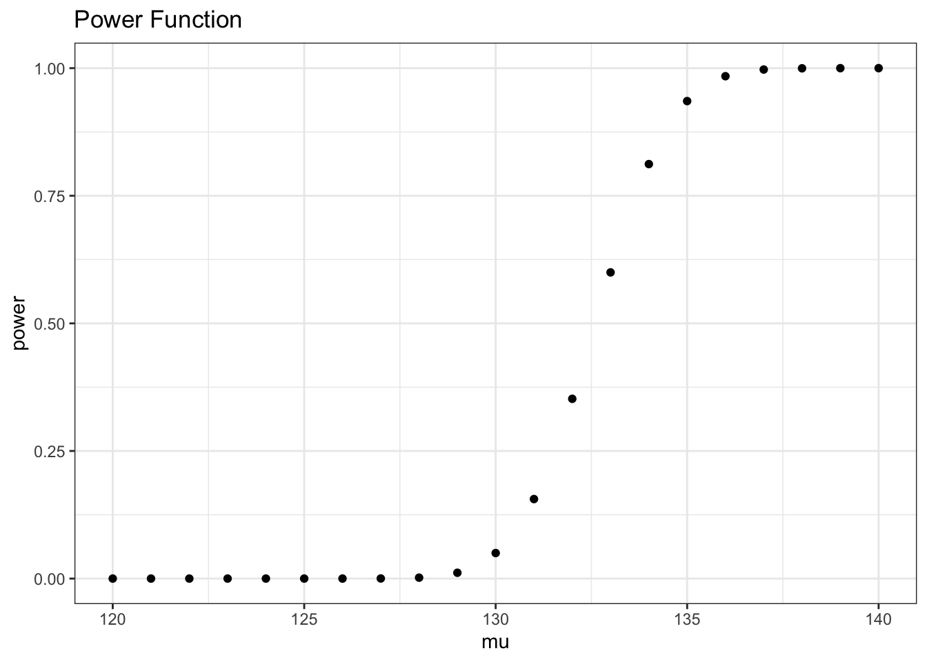
Our intuitions were correct here; power increases with \(\mu\). It begins to increase around 130 and hits essentially 100 around 135; this means that, if the true mean is 135 or higher, we have a very high probability (near 1) of observing a sample mean within the rejection region (over 132.6).
Last but not least, let’s find the p-value for a general sample mean, \(\bar{x}\). Let’s say that we observed a sample mean greater than 130.
We know that the p-value is the probability of seeing the result or a more extreme result given that the null hypothesis is true. In this case, if the null is true, we know that \(\mu = 130\) and thus \(\bar{X} \sim N(130,\frac{25}{10})\). So, the p-value is the probability that this r.v. is equal to or greater the given \(\bar{x}\) (since we said this sample mean was greater than 130, a more extreme sample mean is on the larger side), which is:
\[P(Z > \frac{\bar{x} - 130}{\frac{5}{\sqrt{1}}}) = \Phi(\frac{\bar{x} - 130}{\frac{5}{\sqrt{10}}})\] So, let’s say we observe a sample mean of \(\bar{x} = 132.6\) (what we used for our rejection region above). We get a p-value of:
\[\Phi(\frac{132.6 - 130}{\frac{5}{\sqrt{10}}})\]
We can easily calculate this in R:
## [1] 0.05004841Interestingly, this value is right at .05, which makes sense because this was the rejection region we set above at the .05 level of significance; it all ties together! We have that 132.6 is the \(95^{th}\) quantile of our null distribution, and thus we use it as the cutoff for our hypothesis test, and see that any value beyond it (larger than it) will produce a p-value less than .05 (leading us to reject).
6.6 Practice
- Let \(X_i \sim N(\mu,90)\) be i.i.d. for \(i = 1, ..., 30\) and for an unknown parameter \(\mu\). Consider the test \(H_0: \mu \leq 10\) vs. \(H_A: \mu > 10\).
- Choose a rejection region such that you have a 0\(\%\) chance of a Type II Error.
Solution: The only way to be absolutely sure that you will never have a Type II error is if you always reject the null. Since a Normal covers all real numbers, your rejection cutoff would have to be \(-\infty\). Therefore, you’ll only reject when you see a value greater than \(-\infty\), which is every single value. Basically, you’re always going to reject, which means you’ll never accidentally NOT reject something! Of course, this is not practical in real life, which unfortunately means that you will have to have some non-zero probability of a Type II (and Type I) error.
- Now let \(\alpha = .05\) (that is, the probability of a Type I error is \(5\%\)). What is the critical region?
First, we should set the rejection region. Well, this means that we want to reject a true null 5 percent of the time. If the null is true, then \(\bar{X} \sim N(10,3)\) by the CLT (remember we pick the value for the null closest to the boundary). So, we need the value that this is greater than only 5\(\%\) of the time. Well, for a Standard Normal, we know:
\[P(Z > 1.645) = .05\]
And we can write \(\bar{X}\) in terms of a standard normal:
\[Z \sim \frac{\bar{X} - 10}{\sqrt{3}}\]
So plugging in yields:
\[P(\frac{\bar{X} - 10}{\sqrt{3}} > 1.645) = .05 \rightarrow P(\bar{X} > 12.849) = .05\]
So 12.849 is our rejection region. If we see a value greater than this, we reject! We could also see this quickly in R:
## [1] 12.84897- Continue to let \(\alpha = .05\). What is the power of this test if \(\mu\), the true parameter, is \(11\)? Leave your answer in terms of \(\Phi\).
Solution: Power is just the probability of rejecting given a specific parameter. In this case, we know we are rejecting if \(\bar{X} > 12.849\), and given the information in the prompt we know \(\bar{X} \sim N(11,3)\). So, we just need the probability that \(\bar{X}\) is greater than 12.849!
\[P(\bar{X} > 12.849) = P(\frac{\bar{X} - 11}{\sqrt{3}} = Z > \frac{12.849 - 11}{\sqrt{3}})\]
This is \(1 - \Phi(\frac{12.849 - 11}{\sqrt{3}})\), which we can easily find in R:
## [1] 0.1428684- Continue to let \(\alpha = .05\). Find the general power function (for a general \(\mu\)), in terms of \(\Phi\).
Solution: We could do a bunch of work again, or we could realize that just plugging in \(\mu\) for what we solved in the last problem would work. We want to plug this in for 11. This gives:
\[1 - \Phi(\frac{12.849 - \mu}{\sqrt{3}})\]
We can plot this in R:
x <- seq(from = 0, to = 20, by = 1)
y <- 1 - pnorm((12.849 - x) / sqrt(3))
data <- data.table(x = x, y = y)
ggplot(data, aes(x = x, y = y)) +
  geom_point() +
  theme_bw() +
  xlab("mu") + ylab("power") + ggtitle("Power of our Test")
Clearly, we have an increasing function of \(\mu\); note that this hits a power of \(.5\) when \(\mu\) is \(12.849\) (well, we don’t have \(12.849\) on this chart, just the integers, but you can extrapolate!). This makes sense, since if the true mean is right at the ‘rejection cutoff’, we have a 50/50 chance of being above or beneath the cutoff (and thus rejecting or not rejecting).
- Let \(Y_1,...,Y_n \sim Expo(\lambda)\), where each \(Y_i\) is independent. Consider the test \(H_0: \lambda = \lambda_0\) and \(H_A: \lambda \neq \lambda_0\).
- Find the Likelihood Ratio Test Statistic.
Solution: We can first find the likelihood of the exponential:
\[\prod_{i=1}^n \lambda e^{-\lambda y_i} = \lambda^n e^{-\lambda \sum_{i=1}^n y_i}\]
To maximize this at the null space, we just plug in \(\lambda_0\). To maximize this at the alternative space, we maximize at \(\hat{\lambda}_{MLE}\). So, we get:
\[\frac{\lambda_0^n e^{-\lambda_0 \sum_{i=1}^n y_i}}{\hat{\lambda}_{MLE}^n e^{-\hat{\lambda}_{MLE} \sum_{i=1}^n y_i}}\]
Technically, if \(\lambda_0 = \hat{\lambda}_{MLE}\), we can see that the LRT statistic is just 1.
- Find the Score Test statistic.
Solution: We found the likelihood, so we need the log likelihood and we need to derive that. The log likelihood is:
\[nlog(\lambda) - \lambda \sum_{i=1}^n y_i\]
And the derivative of this w.r.t. \(\lambda\) is the score function:
\[U(\lambda) = \frac{n}{\lambda} - \sum_{i=1}^n y_i\]
We also have to find Fisher’s information. We can take a second derivative of the log likelihood:
\[\frac{-n}{\lambda^2}\]
And the negative expectation of this is just:
\[I(\lambda) = -E(-\frac{n}{\lambda^2}) = \frac{n}{\lambda^2}\]
And now we can plug these two together to get the Score test statistic:
\[U(\lambda_0)^2 I^{-1}(n) = (\frac{n}{\lambda_0} - \sum_{i=1}^n y_i)^2\frac{\lambda_0^2}{n}\]
- Find the Wald Test statistic.
Solution: We’ve already found Fisher, so this is easy:
\[(\hat{\lambda} - \lambda)^2\frac{n}{\hat{\lambda}^2}\]
Where \(\hat{\lambda\) is the MLE.