11 Week 4: Species Distribution Models
11.1 Species Distribution Modeling (SDMs)
Species distribution modeling (SDM) is the application of stastistical methods to predict species occurrence, niche availability, or habitat suitability. In this class, we will focus on the most common version, correlative, which uses species distribution data for model fitting and prediction. This method type contrasts with mechanistic models that are parameterized by how environmental conditions affect fitness or components of fitness such as growth and reproduction.
Correlative SDMs extrapolate from known occurrence data paired with environmental predictors such as temp, precip, and land cover to generate a species-environment model that can be applied to areas without occurrence data. They can also be used to predict changes in distributions such as invasion or with environmental shifts such as climate change.
We will work through four different types of models in this tutorial. For your exercise, you will conduct a Maximum Entropy (MaxEnt) model as well as one other type.
11.2 Background Points and Psuedo-Absences
As we discussed in lecture, if we don’t have true presence-absence data generated through rigorous surveys, we need to consider either the environmental backdrop by considering background points (for MaxEnt) or generate pseudo-absences to treat similarly to absences (for generalized linear models and random forest). The goal when generating background points is to represent the range of environmental conditions available to the species. The goal when generating pseudo-absences is to mimic true absences as closely as possible. Generating either can be challenging to do while both minimizing biases and creating a useful model.
Random Selection: The default option for both background point and pseudo-absence generation is to select points at random from your spatial extent, although conceptually your pseudo-absences should not be at the same point locations as your presences.
Target-Group Background: An option for pseudo-absence generation is to select areas that have been sampled for similar species. In other words, if people have observed a similar species at a location but not the species you are modeling, that is more likely to be a true absence than a simple random point.
Bias File: An option for MaxEnt to include a bias file which is a raster layer of relative sampling effort or likelihood of observation for your species. Background points can then be drawn based on weighting from the bias file to minimize conflating sampling effort with habitat suitability.
There are a variety of other methods that can apply to any data even if you don’t have a good idea of sampling bias. For example, you can spatially thin occurrence points to prevent too much influence from one area (potentially at the expense of statistical power).
11.3 Choosing an SDM framework
It can be challenging to decide which SDM framework to apply, but I think two useful considerations are:
Data type: If you have presence-only data and little insight into how to generate unbiased pseudo-absence points, then MaxEnt might be your preferred starting point. If you have actual presence-absence data then consider a model that uses those absences explicitly such as a GLM, random forest, BRT, or any other conventional framework. Generally, it is more powerful to use true absences if you have them. If you have reasonable but incomplete insight into generating pseudo-absences then the choice may not be as clear just from data type.
Balancing accuracy and interpretability: Conventional linear model frameworks such as GLMs will have the clearest interpretable relationships with classic effect sizes and p-values. However, they will likely have lower predictive accuracy since both MaxEnt and random forest can incorporate complex, non-linear interactions with your species and environment. MaxEnt in particular generates relative habitat suitability metrics by default instead of probability of species occurrence, which can be a bit less clear to interpret and compare with other models.
library(rgbif)
library(dismo) # SDM package
library(rJava) # Java for MaxEnt. If this doesn't install properly, download the proper Java Development Kit for your OS and bit version here: https://www.oracle.com/java/technologies/downloads/?er=221886
library(raster)
library(sf)
library(ggplot2)
library(geodata)
library(terra)
library(spatstat)
library(pROC) # Calculates ROC for GLM
library(MASS)
library(randomForest) # Random forest package
11.4 Basic MaxEnt Walkthrough
MaxEnt (Maximum Entropy) predicts habitat suitability for a species based on presence-only data.
First, let’s bring in some data from GBIF for the lone star tick:
species_name <- "Amblyomma americanum "
gbif_data <- occ_search(scientificName = species_name, limit = 200, hasCoordinate = TRUE)
occs <- gbif_data$data[, c("decimalLongitude", "decimalLatitude")]
head(occs)
## # A tibble: 6 × 2
## decimalLongitude decimalLatitude
## <dbl> <dbl>
## 1 -94.5 37.0
## 2 -83.9 30.5
## 3 -81.7 29.3
## 4 -97.7 26.2
## 5 -82.3 28.6
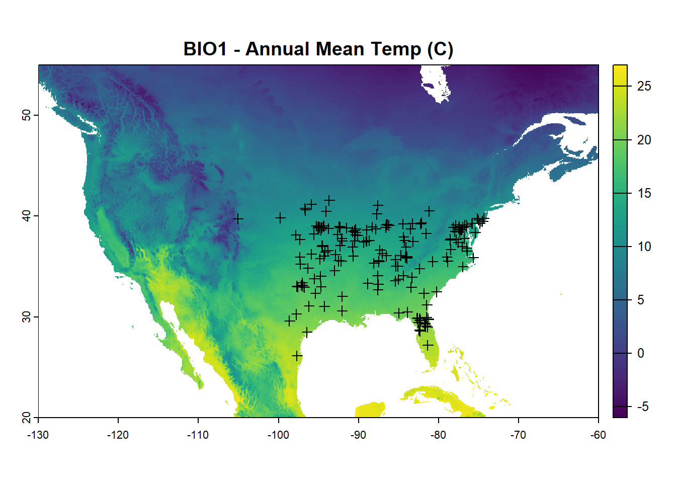
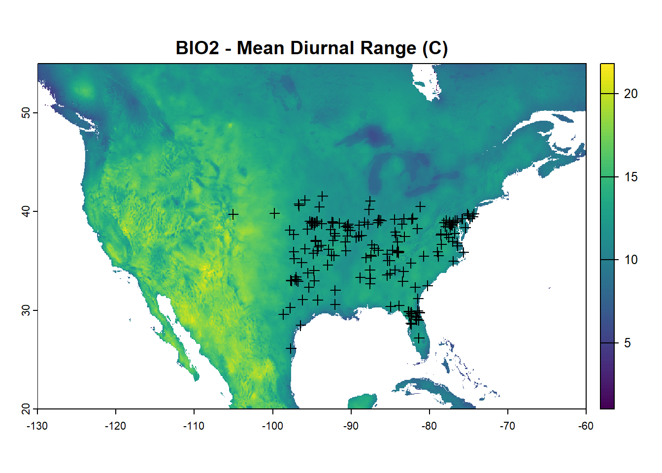
## 6 -81.6 29.1occs_sp <- SpatialPointsDataFrame(coords = occs, data = data.frame(occs), proj4string = CRS("+proj=longlat +datum=WGS84"))Download the worldclim data, which contains 19 different bioclimatic variables. The data are available at different resolutions as well as future climate projections. The data are global in coverage. This may take a bit of time, but you should see the progression of the .zip file being downloaded in a different window.
bioclim_data <- worldclim_global(var = "bio", res = 2.5, path = tempdir())
na_extent <- ext(-130, -60, 20, 55)  # North America extent
bioclim_na <- crop(bioclim_data, na_extent)
Plot the worldclim data (just the first two rasters) and lone star tick points:
 Convert worldclim data into a raster stack for analysis
Create background points randomly across the raster stack
set.seed(4594) # Set seed for random points for reproducibility
background_points <- randomPoints(clim, 200)
plot(bioclim_na[[1]], main = "BIO1 - Annual Mean Temp (C)")
points(background_points, pch = 21) 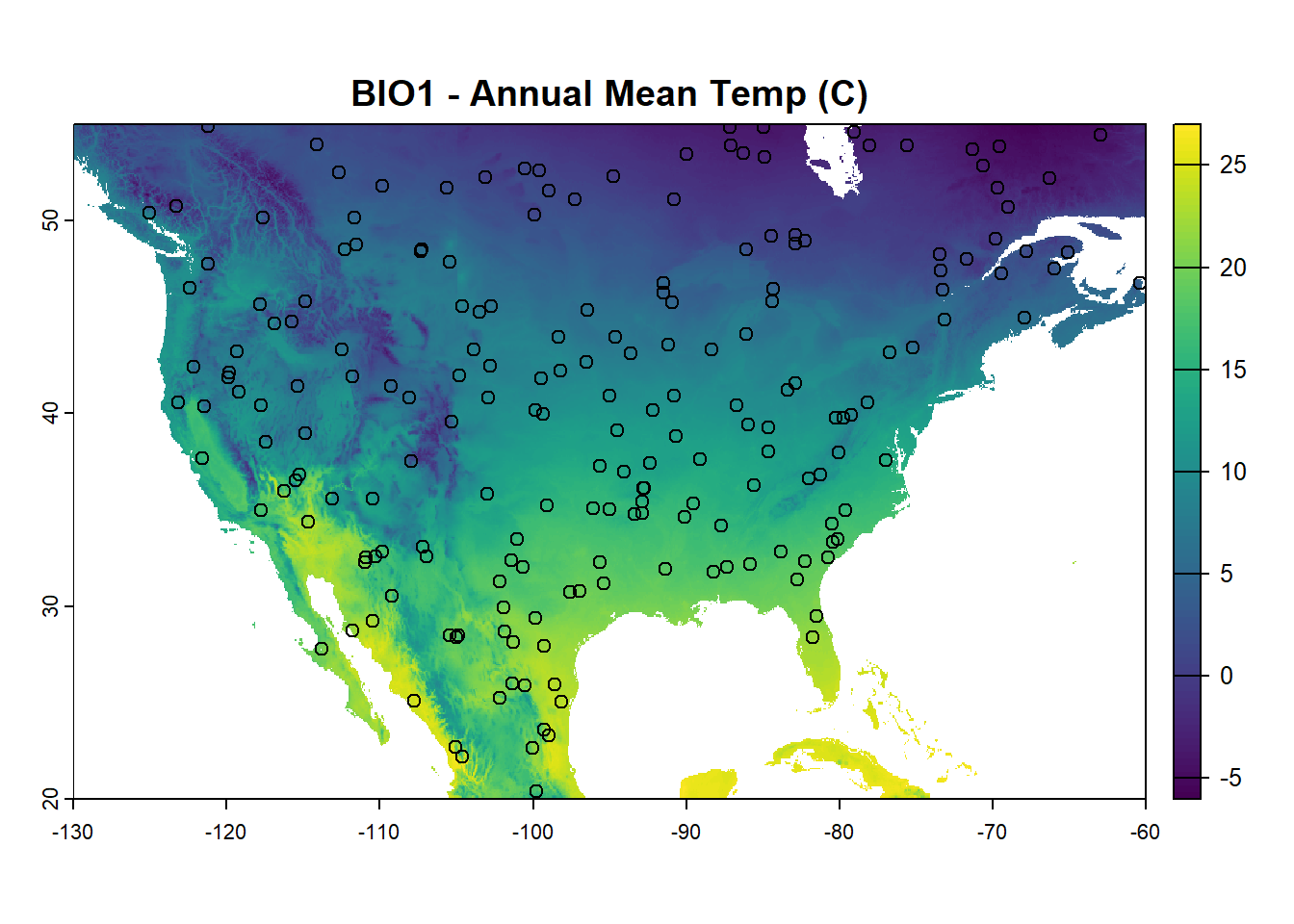
Run the basic maxent() model that requires three components: (1) your raster stack of predictors, (2) your presence-only points, and (3) your background points (in this case randomly selected).
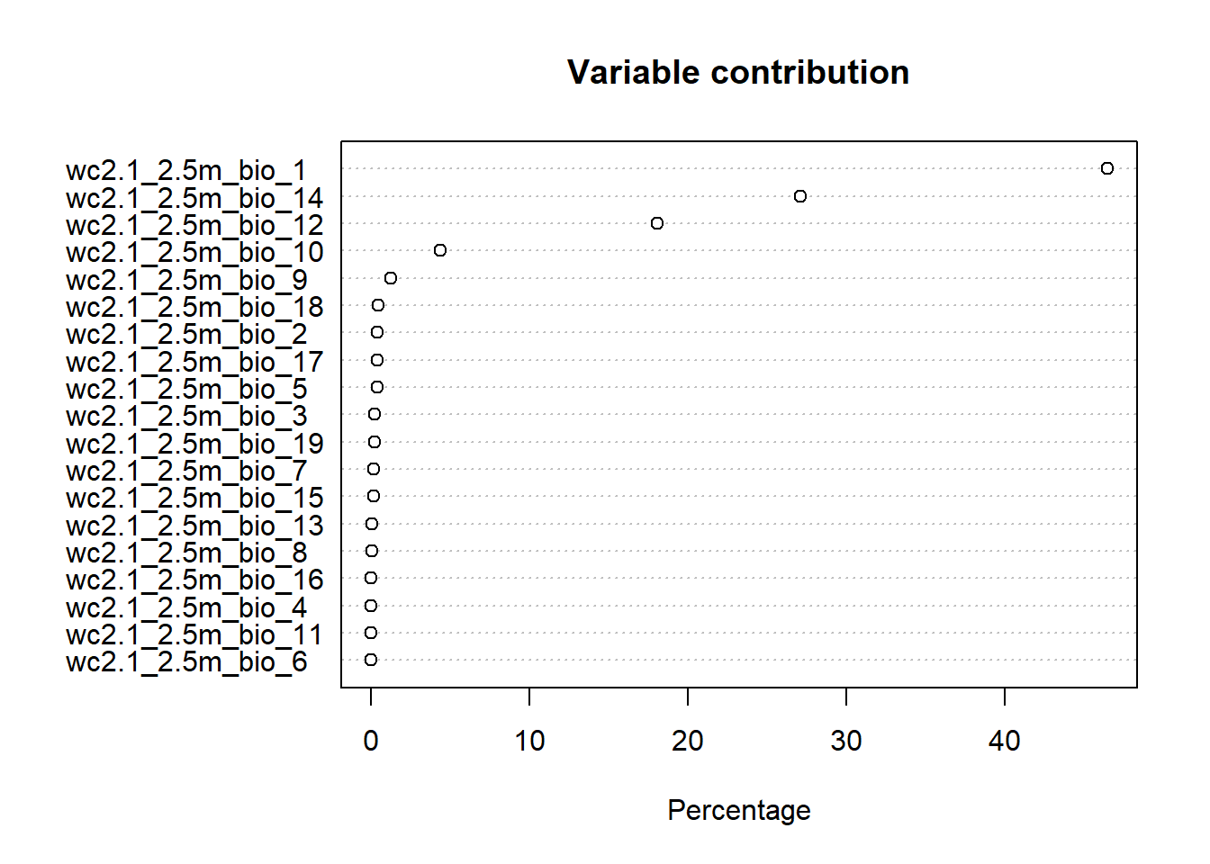
Plot variable contributions from the MaxEnt model fit:
Visualize the environmental constraints determined by MaxEnt. Here I am plotting just the first 6 for visibility, but there are more in the clim stack.
## Visualizing Fitted Constraints from MaxEnt Model
par(mfrow = c(2, 3))
response_curves <- response(maxent_model, names(clim)[1:6])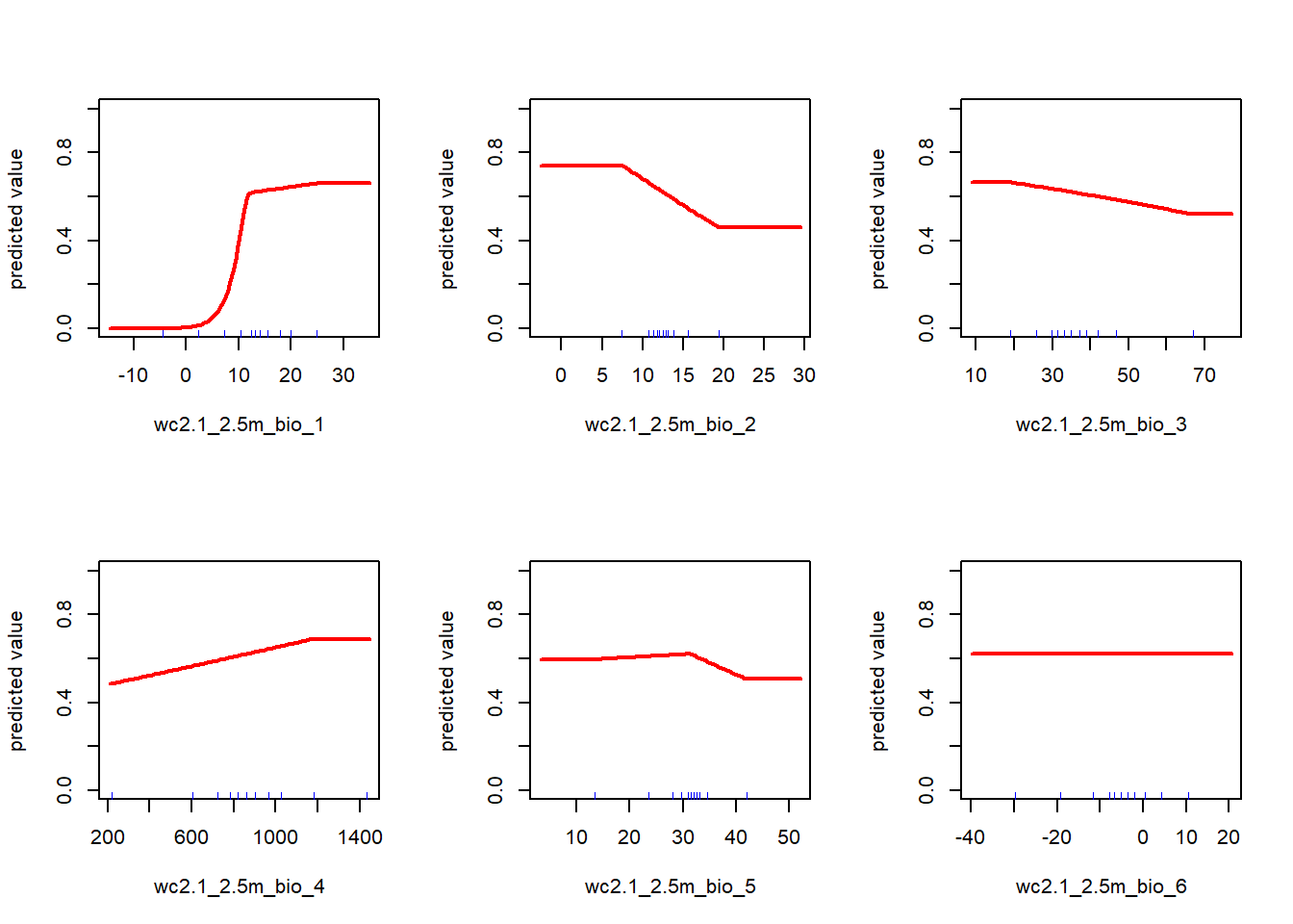
Use your MaxEnt model to predict suitability across your target spatial extent. Note that this one is fitting North America at a relatively fine scale so will take some time. Each raster cell requires prediction so if this takes a long time for you, you may want to limit your raster resolution or spatial extent.
predict_suitability <- predict(maxent_model, clim)
plot(predict_suitability, main="MaxEnt Predicted Suitability for Lone Star Tick")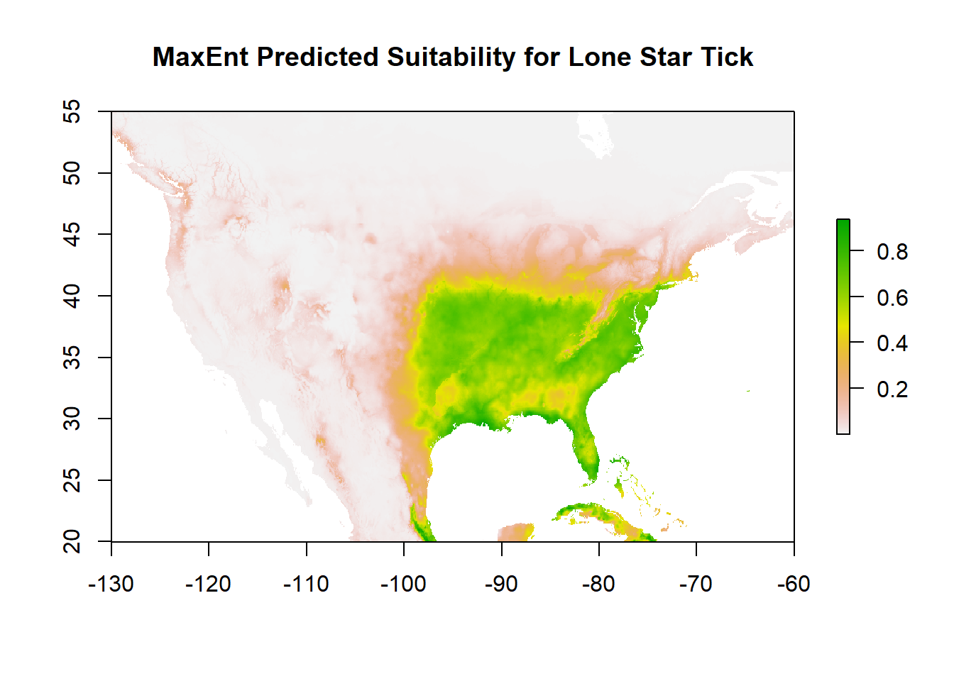
11.4.1 Area Under the Curve (AUC)
Area Under the Curve (AUC) is a metric to evaluate the performance of classification models such as is a species present or absent at a point. The “area” is under the Receiver Operating Characteristic (ROC) curve. An ROC curve plots the true positive rate (sensitivity) against the false positive rate (1 - specificity) at various thresholds. Rules of thumb:
AUC of 0.5 = random chance model (true positives = false positives)
AUC of 0.8 to 1 = model has good to excellent performance in determining true positives vs. false positives.
AUC very close to 1 = look closely for overfitting
AUC is still the most common performance metric for MaxEnt models even though this interpretation is a bit shakey since we are now making assumptions about background points lacking the species presence.
AUC using model occurrences and background points:
auc <- dismo::evaluate(model = maxent_model, p=occs_sp@coords, a=background_points, x = clim)
plot(auc, 'ROC')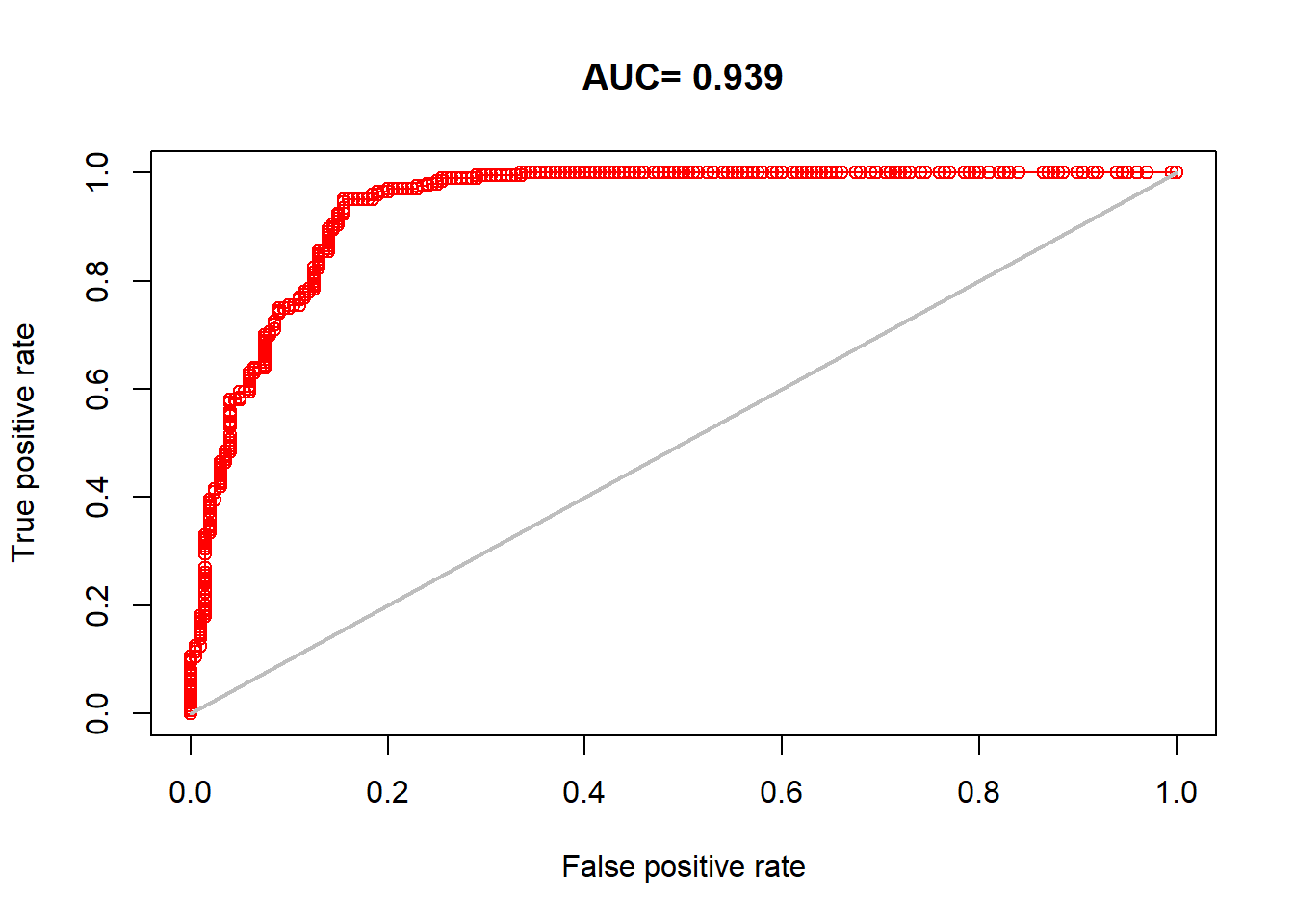
## [1] 0.9385That’s a great AUC result, but are we overrepresenting how good of a fit our model is by looking at the fit of our training data. Training data are the data that the model actually “sees”.
11.4.2 Test/Train Splitting
In many modeling frameworks, you may want to split your data into a training set to train a model and a testing set that validates the model with data it never sees. An extension of this is cross-validation, which validates by looping through multiple testing and training data splits. For this exercise, we will just focus on creating random training and testing data sets. In SDMs, there are methods to create spatially blocked or checkerboard testing and training data splits as well.
First, we will split the data into 5 “folds”, or equal parts. So, 5 folds with create 20% data partitions. We will test on the fold randomly labeled “1” occtest and train on the other folds 2-5 occtrain:
We can then re-run our lone star tick model with just the 80% training subset:
We can then re-run our AUC test but instead use the occurrences we reserved for testing that the model never saw:
auc_test <- dismo::evaluate(model = train_model, p=occtest@coords, a=background_points, x = clim)
plot(auc_test, 'ROC')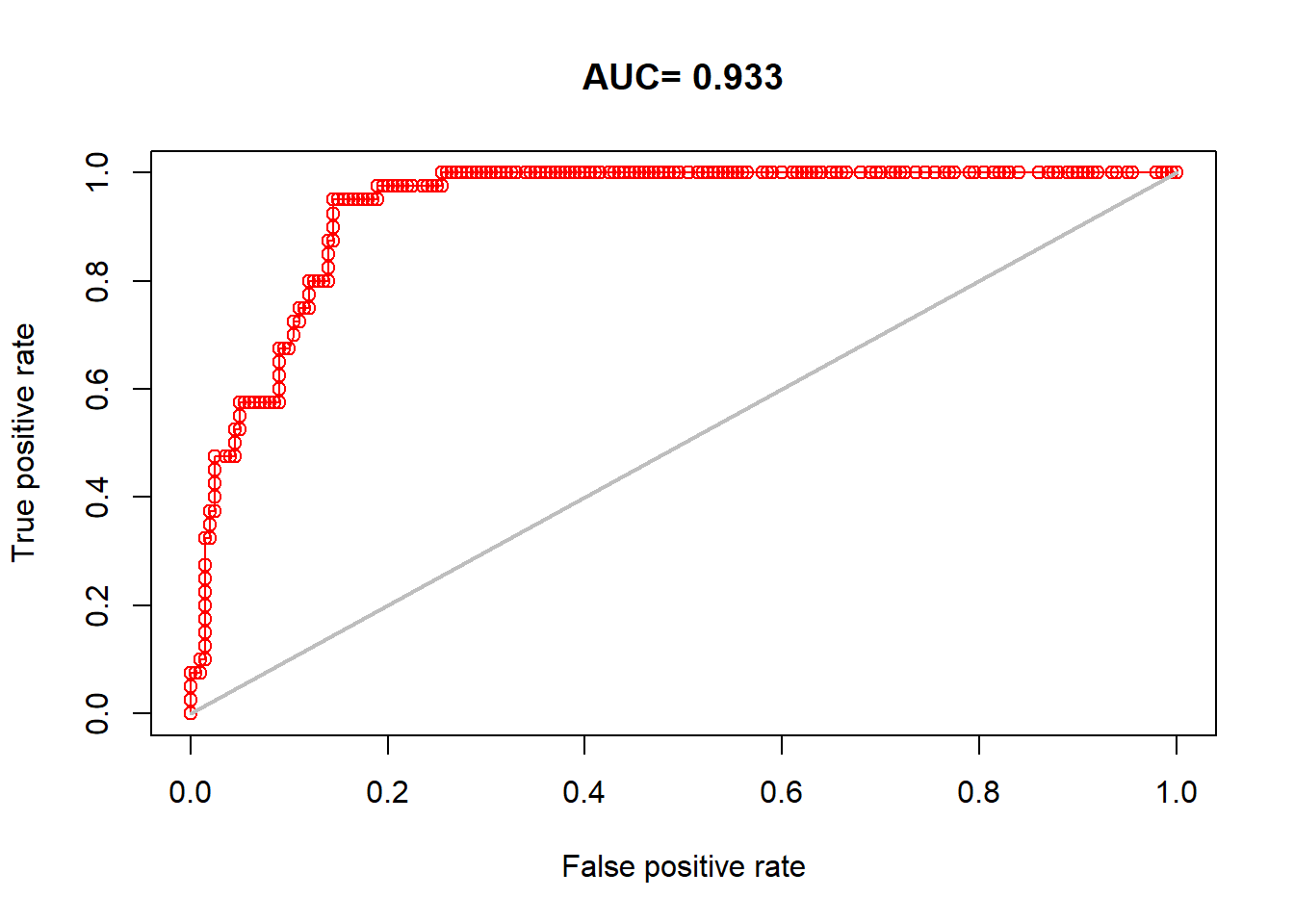
## [1] 0.93275This still looks great. But note that we have one other component in our MaxEnt model that was also included in our model fitting, the background points. For the most honest validation, we will also want to generate random background points again in the same fashion to go along with our testing data:
set.seed(45698)
background_test <- randomPoints(clim, 200)
train_model <- maxent(clim, occtrain, a = background_points)
auc_test <- dismo::evaluate(model = train_model, p=occtest@coords, a=background_test, x = clim)
plot(auc_test, 'ROC')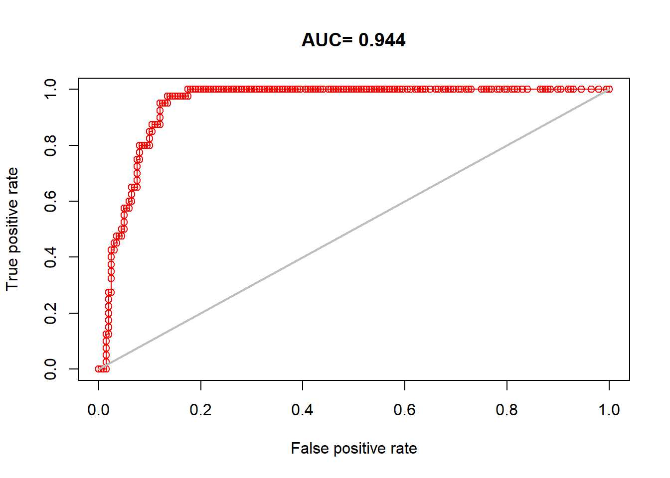
## [1] 0.94425Our model still performs very well.
11.5 A bad MaxEnt model
Let’s try a “bad” MaxEnt model, and create a model based on mallards in Florida to predict mallard in Michigan
species_name_2 <- "Anas platyrhynchos"
gbif_data_2 <- occ_search(scientificName = species_name_2, limit = 50, hasCoordinate = TRUE, stateProvince = "Florida")
occs_2 <- gbif_data_2$data[, c("decimalLongitude", "decimalLatitude")]

occs_sp_2 <- SpatialPointsDataFrame(coords = occs_2, data = data.frame(occs_2), proj4string = CRS("+proj=longlat +datum=WGS84"))
species_name_2 <- "Anas platyrhynchos"
gbif_data_3 <- occ_search(scientificName = species_name_2, limit = 50, hasCoordinate = TRUE, stateProvince = "Michigan")
occs_3 <- gbif_data_3$data[, c("decimalLongitude", "decimalLatitude")]
mall_test <- SpatialPointsDataFrame(coords = occs_3, data = data.frame(occs_3), proj4string = CRS("+proj=longlat +datum=WGS84"))mall_mod <- maxent(clim, occs_sp_2, a = background_test)
predict_suitability2 <- predict(mall_mod, clim)
plot(predict_suitability2, main="Mallard Suitability based on Florida")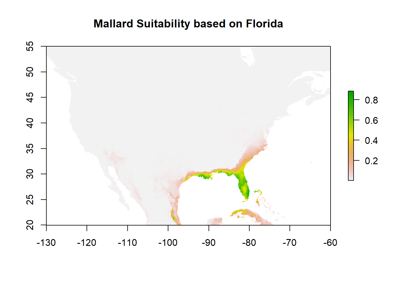
auc_test <- dismo::evaluate(model = mall_mod, p=mall_test@coords, a=background_points, x = clim)
plot(auc_test, 'ROC')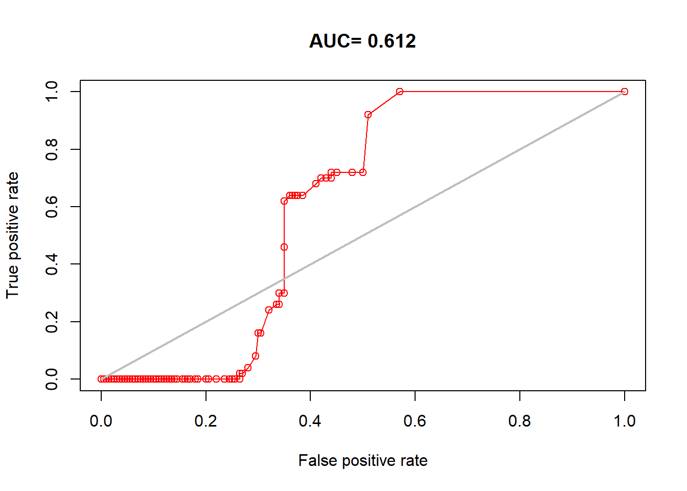
## [1] 0.611611.6 GLM version
For a generalized linear model (GLM), we have to convert the background points to pseudo-absences (i.e., true 0’s for a binary logistic regression). The poorest way is to just do this randomly and use the same background points as the MaxEnt.
occ_values <- terra::extract(clim, occtrain, df = TRUE)
background_values <- terra::extract(clim, background_points, df = TRUE)

occ_values$presence <- 1
background_values$presence <- 0

data_glm <- rbind(occ_values, background_values)
data_glm <- na.omit(data_glm)  # Remove NA values
We can then fit a GLM model predicting the presence (0/1) based on all variables (presence ~ .). Generally, this is unadvisable without good justification since you risk multicollinearity issues and lose the strength to be testing a hypothesis, but it will generally maximize your accuracy (more variables will always fit better in a GLM, but maybe overfit). Therefore, you will generally want to construct your hypotheses and choose a model that makes biological sense and will be useful for your interpretation:
glm_model <- glm(presence ~ wc2.1_2.5m_bio_1 + wc2.1_2.5m_bio_5 , data = data_glm, family = binomial)
summary(glm_model)
##
## Call:
## glm(formula = presence ~ wc2.1_2.5m_bio_1 + wc2.1_2.5m_bio_5,
## family = binomial, data = data_glm)
##
## Coefficients:
## Estimate Std. Error z value Pr(>|z|)
## (Intercept) -1.60352 1.53343 -1.046 0.295698
## wc2.1_2.5m_bio_1 0.15521 0.04337 3.579 0.000345 ***
## wc2.1_2.5m_bio_5 -0.01851 0.06419 -0.288 0.773137
## ---
## Signif. codes: 0 '***' 0.001 '**' 0.01 '*' 0.05 '.' 0.1 ' ' 1
##
## (Dispersion parameter for binomial family taken to be 1)
##
## Null deviance: 494.61 on 359 degrees of freedom
## Residual deviance: 437.75 on 357 degrees of freedom
## AIC: 443.75
##
## Number of Fisher Scoring iterations: 4You can see we now have effect sizes and p-values. Here, we can say BIO1 has a significant effect and not BIO5.
We can then make predictions from our raster and plot:
predicted_raster <- predict(bioclim_na, glm_model, type = "response")
plot(predicted_raster, main = "Predicted Lone Star Tick Prob. from GLM")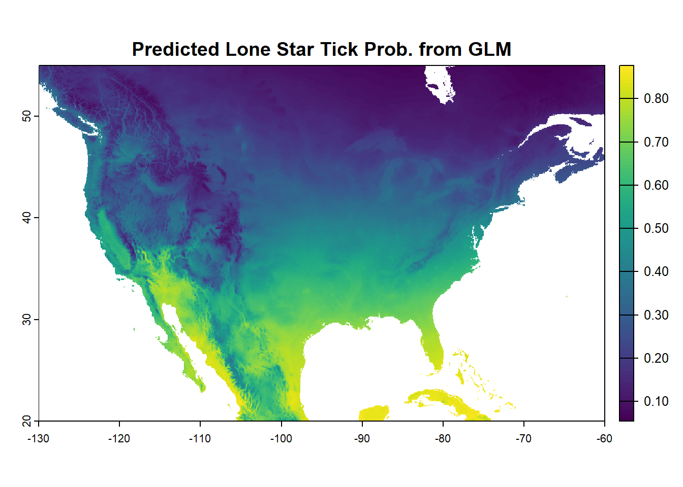
Create test values from above to test our model using UNSEEN validation data:
test_values <- terra::extract(clim, occtest, df = TRUE)
background_test2 <- terra::extract(clim, background_test, df = TRUE)

test_values$presence <- 1
background_test2$presence <- 0

data_glm_test <- rbind(test_values, background_test2)
data_glm_test <- na.omit(data_glm_test)  # Remove NA values
Again check out the AUC based on the test data:
glm_pred <- predict(glm_model, newdata = data_glm_test, type = "response")
glm_auc <- roc(data_glm_test$presence, glm_pred)
plot(glm_auc, main="ROC Curve for GLM Model")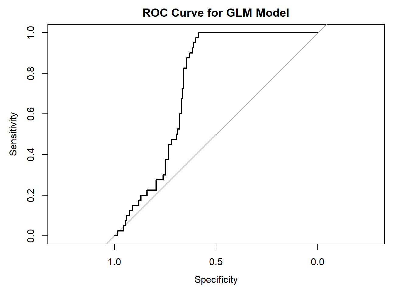
## Area under the curve: 0.7378And compare to the MaxEnt model using the same data:
comparison_metrics <- data.frame(
  Model = c("MaxEnt", "GLM"),
  AUC = c(auc@auc, glm_auc$auc)
)

ggplot(comparison_metrics, aes(x=Model, y=AUC, fill=Model)) +
  geom_bar(stat="identity") +
  theme_minimal() +
  ggtitle("AUC Comparison: MaxEnt vs. GLM")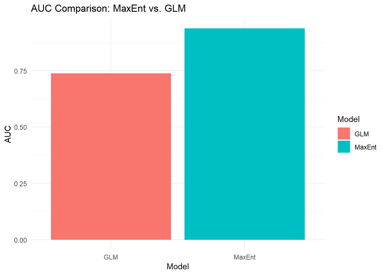
11.7 Random Forest
Another flexible machine learning option is random forest which creates a forest of classification trees. Generally, this approach is best when trying to optimize for prediction accuracy at the expense of interpretability and hypothesis testing (although there are some ways to still compare variable importance and impact).
A random forest can be run either as a regression or for categorization. We will set the presence absence data from above as.factor() to run a binary classification version:
# Fit the randomForest model using all predictors, removing the ID column 1
rf_model <- randomForest(as.factor(presence) ~ ., data = data_glm[,-1], importance = TRUE)
print(rf_model)
##
## Call:
## randomForest(formula = as.factor(presence) ~ ., data = data_glm[, -1], importance = TRUE)
## Type of random forest: classification
## Number of trees: 500
## No. of variables tried at each split: 4
##
## OOB estimate of error rate: 14.72%
## Confusion matrix:
## 0 1 class.error
## 0 163 37 0.185
## 1 16 144 0.100The output here is an out of bag (OOB) estimate of error, which pools error from each individual tree run on the unseen data from those trees. We also see a confusion matrix which tells us how often in our training data that a 1 is classified as a 1 and a 0 and a 0, as well as the wrong classes.
Instead of parameter estimates like a GLM, we can look at variable importance in two main ways. (1) Mean % decrease of accuracy, which is the reduction in model accuracy if that variable is randomly permutated (i.e., made uninformative). (2) Mean decrease Gini which is a calculation based on how important a variable is in splitting data within trees.
##                            0        1 MeanDecreaseAccuracy MeanDecreaseGini
## wc2.1_2.5m_bio_1  11.5538201 17.62114             19.98931        18.841658
## wc2.1_2.5m_bio_2   3.7513382 11.82603             11.79225         6.728797
## wc2.1_2.5m_bio_3   5.1575792 15.20207             16.13048         6.658454
## wc2.1_2.5m_bio_4   2.2359345 12.78727             14.50425         5.293104
## wc2.1_2.5m_bio_5   9.5817738 12.94766             15.88492        10.316460
## wc2.1_2.5m_bio_6   3.9116546 12.35706             12.76804         6.294155
## wc2.1_2.5m_bio_7  -1.5588565 12.47505             12.90904         3.993956
## wc2.1_2.5m_bio_8   0.7010351 12.04033             11.49099         5.024846
## wc2.1_2.5m_bio_9   2.9526966 12.13963             13.23270         5.869853
## wc2.1_2.5m_bio_10  9.3127808 21.82688             21.95722        20.100342
## wc2.1_2.5m_bio_11  6.2987281 14.88359             16.35827         9.805163
## wc2.1_2.5m_bio_12  7.3545411 16.83147             17.55091        18.522794
## wc2.1_2.5m_bio_13  4.7903256 11.80371             13.77860         9.273847
## wc2.1_2.5m_bio_14  6.5123068 12.15875             14.15920         7.836027
## wc2.1_2.5m_bio_15  2.2958661 15.27602             16.05678         7.127344
## wc2.1_2.5m_bio_16  5.1925485 11.26621             12.31771         9.470185
## wc2.1_2.5m_bio_17  6.5503448 12.33705             13.58421        11.454252
## wc2.1_2.5m_bio_18  3.1517770 14.84910             14.33677         9.362653
## wc2.1_2.5m_bio_19  2.8783373 12.10052             12.45852         5.381335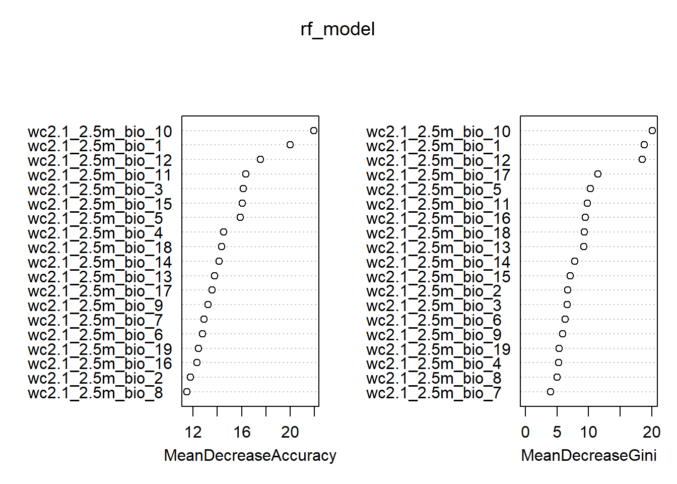
We can again still make predictions from this in terms of probability of occurrence:
And plot:
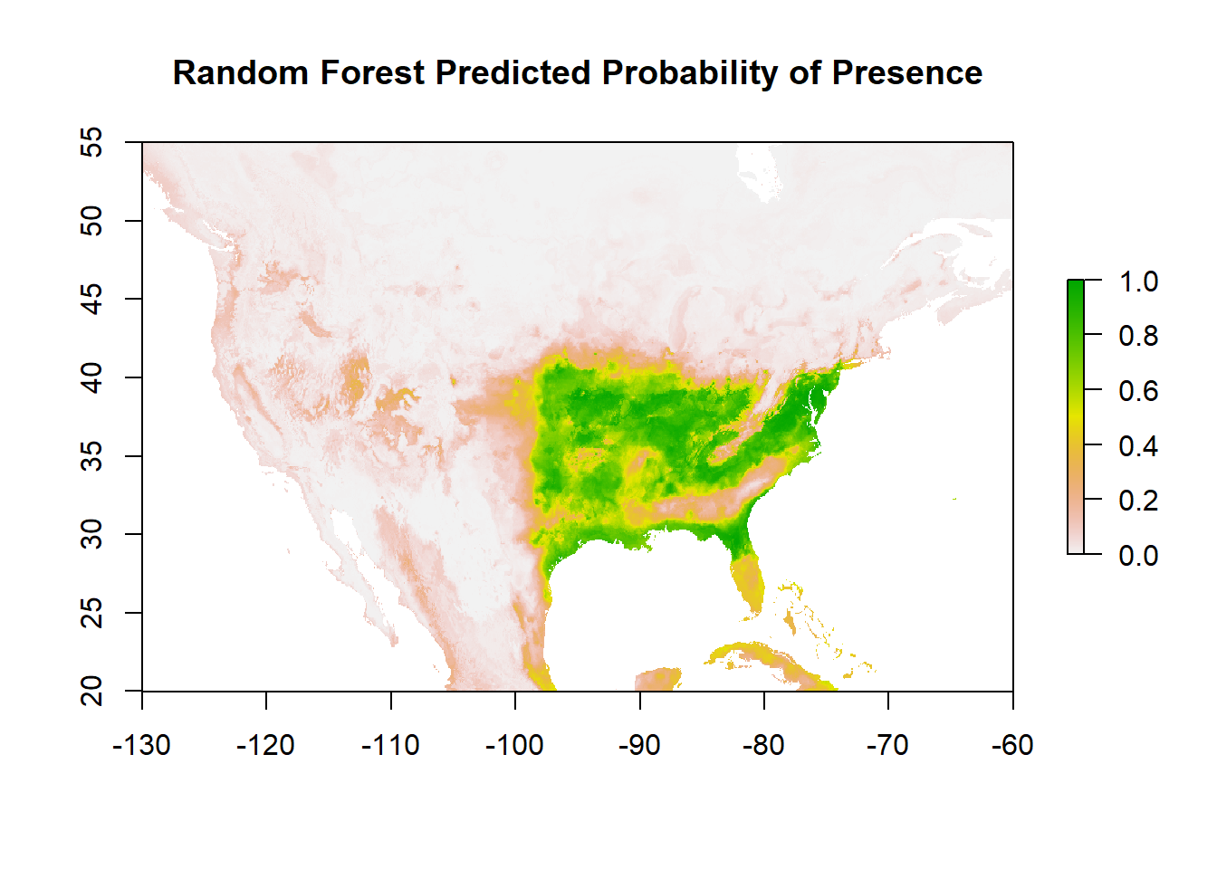
Calculate the AUC based on the UNSEEN test data:
rf_pred <- predict(rf_model, newdata = data_glm_test[,-1], type = "prob")[, 2]
rf_auc <- roc(data_glm_test[,-1]$presence, rf_pred)
print(rf_auc$auc)
## Area under the curve: 0.9399And do our comparison of AUC for all 3 SDM types:
comparison_metrics <- data.frame(
  Model = c("MaxEnt", "GLM", "RF"),
  AUC = c(auc@auc, glm_auc$auc, rf_auc$auc)
)
ggplot(comparison_metrics, aes(x = Model, y = AUC, fill = Model)) +
  geom_bar(stat = "identity") +
  theme_minimal() +
  ggtitle("AUC Comparison: MaxEnt vs. GLM vs. RF") +
  ylim(0, 1)  # set limits to the probability range (0-1)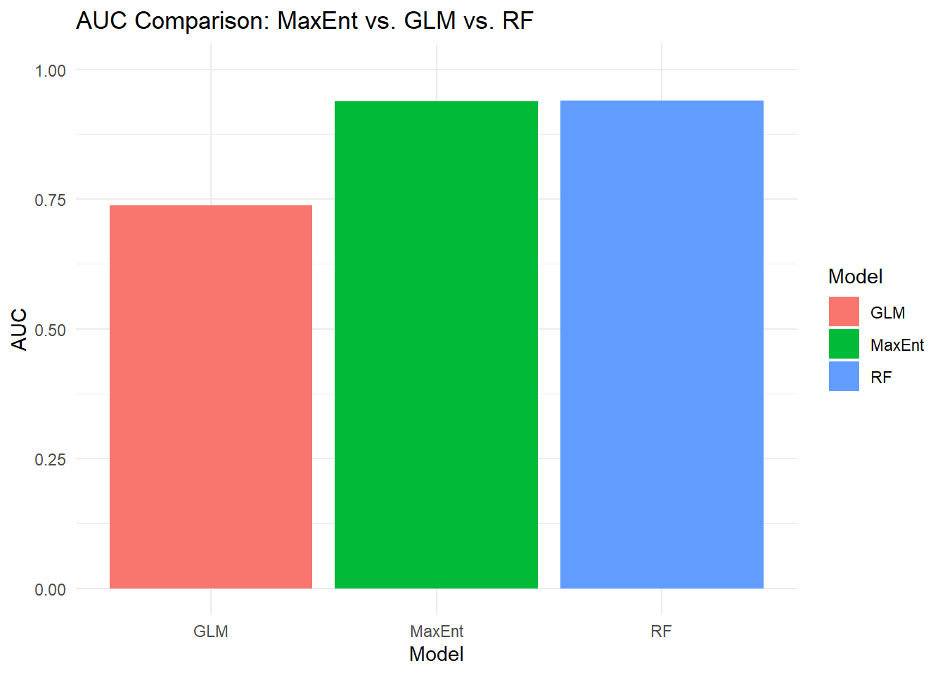
11.8 Extensions
11.8.1 Worldclim projections
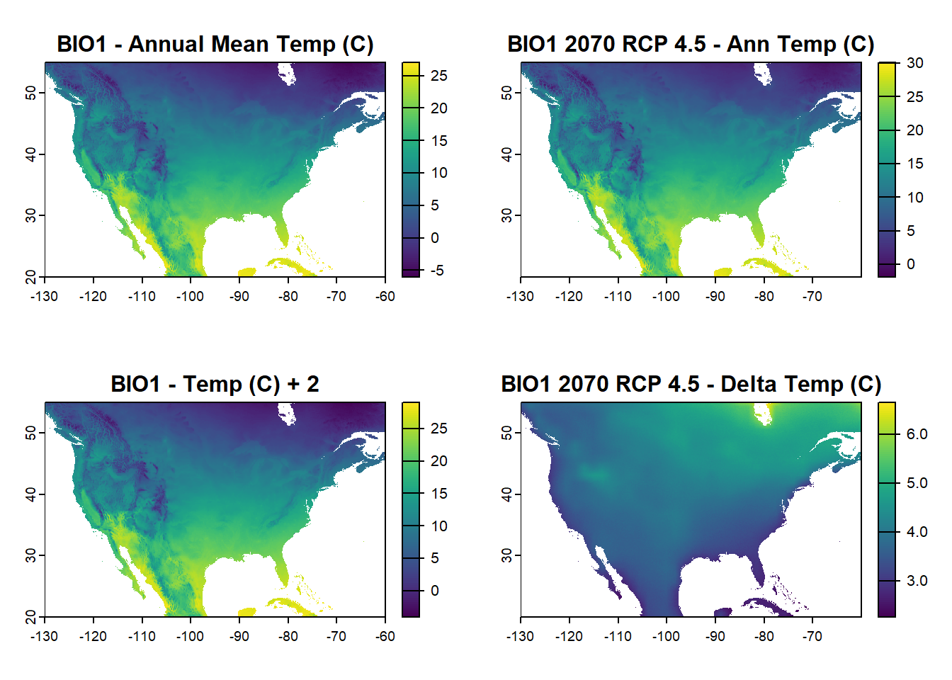
You can also bring in worldclim data for projections in the future under different RCP scenarios, e.g. 2070 under RCP 4.5 or. Or, manually add a fixed value such as 2 degrees C to the entire raster (including your own). Note that this was updated on Feb 16th, 2025 since the package/function changed since I first designed this exercise.
# Updated code for brining in a 2070 climate scenario. There are different models and scenarios you can check out under the function description
future2070 <- cmip6_world(var = "bioc", res = 2.5, model = "ACCESS-CM2", ssp = 245, time = "2061-2080", path = tempdir())
na_extent <- ext(-130, -60, 20, 55)  # North America extent
future_na <- crop(future2070, na_extent)

# Manual add 2 to the original annual temperature raster from the exericse
manual_temp <- bioclim_na[[1]] + 2

# Calculate difference between the 2070 and current climate model for the annual temperature raster
temp_change <- future_na[[1]] - bioclim_na[[1]]

# Plot to show current annual temp, future annual temp, the manual difference raster, and the difference between current and future
par(mfrow=c(2,2))
plot(bioclim_na[[1]], main = "BIO1 - Annual Mean Temp (C)")
plot(future_na[[1]], main = "BIO1 2070 RCP 4.5 - Ann Temp (C)")
plot(manual_temp, main = "BIO1 - Temp (C) + 2")
plot(temp_change, main = "BIO1 2070 RCP 4.5 - Delta Temp (C)")