Listing 1.1: Rolling two dice: pb
#> New names:
#> • `` -> `...1`
#> • `` -> `...2`Definition 1.1 “A probability is simply a number between 0 and 1 that measures the uncertainty of a particular event.” (Albert and Hu, 2019, p. 17) (pdf)
Only applicable when the outcomes are equally likely.
\[Prob(Outcome) = \frac{1}{\text{Number of outcomes}} \tag{1.1}\]
Classical View: What is the probability of rolling doubles with two dice?
There are \(6 \times 6 = 36\) equally likely ways of rolling two distinguishable dice and there are exactly six ways of rolling doubles. So using the classical viewpoint, the probability of doubles is \(\frac{6}{36} = \frac{1}{6} = 0.1666667\).
Applicable when it is possible to repeat the random experiment many times under the same conditions.
Frequency View: What is the probability of rolling doubles with two dice?
Imagine rolling two dice many times under similar conditions. Each time two dice are rolled, we observe whether the result are doubles or not. Then the probability of doubles is approximated by the relative frequency
\[Prob(doubles) \approx \frac{\text{number of doubles}}{\text{number of experiments}}\]
Listing 1.1: Rolling two dice: pb
#> New names:
#> • `` -> `...1`
#> • `` -> `...2`Listing 1.2: Show the simulation result of rolling two dice: pb
str(d)#> tibble [100,000 × 3] (S3: tbl_df/tbl/data.frame)
#> $ Die1 : int [1:100000] 1 1 2 2 1 1 6 2 3 1 ...
#> $ Die2 : int [1:100000] 5 1 4 2 4 5 4 2 1 3 ...
#> $ Match: logi [1:100000] FALSE TRUE FALSE TRUE FALSE FALSE ...The empirical probability of rolling doubles in 10^{5} throws is 0.16841. In contrast: The analytical probability of rolling doubles is 1/6 = 0.1666667.
“What if one can’t apply these two interpretations of probability? That is, what if the outcomes of the experiment are not equally likely, and it is not feasible or possible to repeat the experiment many times under similar conditions?” (Albert and Hu, 2019, p. 23f) (pdf)
Measuring probabilities subjectively: Calibration
Calibrate your subjective believe with an experiment where the probabilities of the outcome are clear, e.g., drawing a certain amounts of red/black balls hidden in a box when you know the general red/black distribution. Compare your bet (feelings) with the balls against the other (really) interesting probability (e.g., Trump will win the next election). Change the ball distribution accordingly so that your bets are getting more precise and compare again with your case you are interested in.
Definition 1.2 “The collection of all outcomes that are possible is the sample space.” (Albert and Hu, 2019, p. 27) (pdf)
Roll two fair dice
Listing 1.3: Indistinguishable dice: Order does not matter = Combination
t(gtools::combinations(6, 2, repeats.allowed = TRUE))#> [,1] [,2] [,3] [,4] [,5] [,6] [,7] [,8] [,9] [,10] [,11] [,12] [,13] [,14]
#> [1,] 1 1 1 1 1 1 2 2 2 2 2 3 3 3
#> [2,] 1 2 3 4 5 6 2 3 4 5 6 3 4 5
#> [,15] [,16] [,17] [,18] [,19] [,20] [,21]
#> [1,] 3 4 4 4 5 5 6
#> [2,] 6 4 5 6 5 6 6Listing 1.4: Distinguishable dice: Order matters = Permutation
t(gtools::permutations(6, 2, repeats.allowed = TRUE))#> [,1] [,2] [,3] [,4] [,5] [,6] [,7] [,8] [,9] [,10] [,11] [,12] [,13] [,14]
#> [1,] 1 1 1 1 1 1 2 2 2 2 2 2 3 3
#> [2,] 1 2 3 4 5 6 1 2 3 4 5 6 1 2
#> [,15] [,16] [,17] [,18] [,19] [,20] [,21] [,22] [,23] [,24] [,25] [,26]
#> [1,] 3 3 3 3 4 4 4 4 4 4 5 5
#> [2,] 3 4 5 6 1 2 3 4 5 6 1 2
#> [,27] [,28] [,29] [,30] [,31] [,32] [,33] [,34] [,35] [,36]
#> [1,] 5 5 5 5 6 6 6 6 6 6
#> [2,] 3 4 5 6 1 2 3 4 5 6There are three ways to record sample spaces:
“… we cannot say that one sample space is better than another sample space. We will see that in particular situations some sample spaces are more convenient than other sample spaces when one wishes to assign probabilities.” (Albert and Hu, 2019, p. 31) (pdf)
The book explains the three different types of assigning probabilities with a girl choosing a dip of ice cream from four different flavors:
“One defines probability as a function on events that satisfies three basic laws or axioms.” (Albert and Hu, 2019, p. 35) (pdf)
\[P(A_{1} \cup A_{2} \cup A_{3}…) = P(A_{1}) + P(A_{2}) + P(A_{3}) + … \tag{1.2}\]
Complement Property:
\[P(\overline{A}) = 1 - P(A) \tag{1.3}\]
Addition Property:
\[P(A \cup B) = P(A) + P(B) - P(A \cap B) \tag{1.4}\]
Please keep in mind that I am a learner! There is no guarantee that my answers are correct.
In the following problems, indicate if the given probability is found using the classical viewpoint, the frequency viewpoint, or the subjective viewpoint.
Joe is doing well in school this semester – he is 90% sure that will receive As in all his classes. SUBJECTIVE
Two hundred raffle tickets are sold and one ticket is a winner. Someone purchased one ticket and the probability that her ticket is the winner is 1/200. CLASSICAL
Suppose that 30% of all college women are playing an intercollegiate sport. If we contact one college woman at random, the chance that she plays a sport is 0.3. CLASSICAL
Two Polish statisticians in 2002 were questioning if the new Belgium Euro coin was indeed fair. They had their students flip the Belgium Euro 250 times, and 140 came up heads. FREQUENCY
Many people are afraid of flying. But over the decade 1987-96, the death risk per flight on a US domestic jet has been 1 in 7 million. FREQUENCY
In a roulette wheel, there are 38 slots numbered 0, 00, 1, …, 36. There are 18 ways of spinning an odd number, so the probability of spinning an odd is 18/38. CLASSICAL
In the following problems, indicate if the given probability is found using the classical viewpoint, the frequency viewpoint, or the subjective viewpoint.
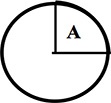
The probability that the spinner lands in the region A is 1/4. CLASSICAL
The meteorologist states that the probability of rain tomorrow is 0.5. You think it is more likely to rain and you think the chance of rain is 3/4. SUBJECTIVE
A football fan is 100% certain that his high school football team will win their game on Friday. SUBJECTIVE
Jennifer attends a party, where a prize is given to the person holding a raffle ticket with a specific number. If there are eight people at the party, the chance that Jennifer wins the prize is 1/8. CLASSICAL
What is the chance that you will pass an English class? You learn that the professor passes 70% of the students and you think you are typical in ability among those attending the class. FREQUENCY
If you toss a plastic cup in the air, what is the probability that it lands with the open side up? You toss the cup 50 times and it lands open side up 32 times, so you approximate the probability by 32/50 FREQUENCY
For the following experiments, a list of possible outcomes is given. Decide if one can assume that the outcomes are equally likely. If the equally likely assumption is not appropriate, explain which outcomes are more likely than others.
Solution: Selecting Marble
Not Equally Likely Outcomes: There are different probabilities for the three colors at the start condition:
After marbles are drawn the probabilities are changing, because there is no replacement. So this is also not a binomial experiment, as explained in (chap-4-binomial-probabilities?).
You observe the gender of a baby born today at your local hospital. Outcomes: {male, female} Equally Likely Outcomes
Your school’s football team is playing the top rated school in the country. Outcomes: {your team wins, your team loses} Not Equally Likely Outcomes: My team wins, because we are the top rated school in the country.
A bag contains 50 slips of paper, Ten slips are assigned to each category numbered 1 through 5. You choose a slip at random from the bag and notice the number on the slip. Outcomes: {1, 2, 3, 4, 5} Equally Likely Outcomes
For the following experiments, a list of possible outcomes is given. Decide if one can assume that the outcomes are equally likely. If the equally likely assumption is not appropriate, explain which outcomes are more likely than others.
You wait at a bus stop for a bus. From experience, you know that you wait, on average, 8 minutes for this bus to arrive. Outcomes: {wait less than 10 minutes, wait more than 10 minutes} Not Equally Likely Outcomes
You roll two dice and observe the sum of the numbers. Outcomes: {2, 3, 4, 5, 6, 7, 8, 9, 10, 11, 12} Equally Likely Outcomes
You get a grade for an English course in college. Outcomes: {A, B, C, D, F} Not Equally Likely Outcomes: Depends on my course work.
You interview a person at random at your college and ask for his or her age. Outcomes: {17 to 20 years, 21 to 25 years, over 25 years} Not Equally Likely Outcomes: Age groups different large, different distribution of ages of students enrolled in colleges
Suppose you flip a fair coin until you observe heads. You repeat this experiment many times, keeping track of the number of flips it takes to observe heads. Here are the numbers of flips for 30 experiments.
x1 <- c(1,3,1,2,1,1,2,6,1,2,1,1,1,1,3,2,1,1,2,1,5,2,1,7,3,3,3,1,2,3)

sum(x1 == 2)
sum(x1 > 2)
median(x1)
#> [1] 7
#> [1] 9
#> [1] 2Approximate the probability that it takes you exactly two flips to observe heads. \(\frac{7}{30} = 0.2333333\)
Approximate the probability that it takes more than two flips to observe heads. \(\frac{9}{30} = 0.3\)
What is the most likely number of flips? Median = 2
You drive to work 20 days, keeping track of the commuting time (in minutes) for each trip. Here are the twenty measurements.
x2 <- c(25.4, 27.8, 26.8, 24.1, 24.5, 23.0, 27.5, 24.3, 28.4, 29.0, 29.4, 24.9, 26.3, 23.5, 28.3, 27.8, 29.4, 25.7, 24.3, 24.2)

sum(x2 < 25.0)
sum(x2 >= 25.0 & x2 <= 28.0)
#> [1] 8
#> [1] 7Approximate the probability that it takes you under 25 minutes to drive to work. \(\frac{8}{20} = \frac{2}{5} = 0.4\)
Approximate the probability it takes between 25 and 28 minutes to drive to work. \(\frac{7}{20} 0.35\)
Suppose one day it takes you 23 minutes to get to work. Would you consider this unusual? Why? Yes, it is unusual because it happened only once in 20 days = 0.05
Consider your subjective probability P(M) where M is the event that the United States will send a person to Mars in the next twenty years.
Let B denote the event that you select a red ball from a box of five red and five white balls. Consider the two bets
• BET 1 – If M occurs (United States will send a person to Mars in the next 20 years), you win $100. Otherwise, you win nothing.
• BET 2 – If B occurs (you observe a red ball in the above experiment), you win $100. Otherwise, you win nothing.
Assign bold to the bet that you prefer.
Let B represent choosing red from a box of 7 red and 3 white balls. Again compare BET 1 with BET 2 – which bet do you prefer?
Let B represent choosing red from a box of 3 red and 7 white balls. Again compare BET 1 with BET 2 – which bet do you prefer?
Based on your answers to (a), (b), (c), circle the interval of values that contain your subjective probability P(M). 50%-70%
Consider your subjective probability P(S) where S is the event that at age 60 you will be living in the same state as you currently live.
Let B denote the event that you select a red ball from a box of five red and five white balls. Consider the two bets
• BET 1 – If S occurs (you live in the same state at age 60 80), you win $100. Otherwise, you win nothing.
• BET 2 – If B occurs (you observe a red ball in the above experiment), you win $100. Otherwise, you win nothing.
Assign bold to the bet that you prefer.
Let B represent choosing red from a box of 7 red and 3 white balls. Again compare BET 1 with BET 2 – which bet do you prefer?
Let B represent choosing red from a box of 3 red and 7 white balls. Again compare BET 1 with BET 2 – which bet do you prefer?
Based on your answers to (a), (b), (c), circle the interval of values that contain your subjective probability P(S) 30%-50%
Suppose you choose a page at random from the book Huckleberry Finn by Mark Twain and find the first vowel on the page.
| Vowel | a | e | i | o | u |
|---|---|---|---|---|---|
| Probability | 0.2 | 0.2 | 0.2 | 0.2 | 0.2 |
| Vowel | a | e | i | o | u |
|---|---|---|---|---|---|
| Probability | 0.3 | 0.3 | 0.15 | 0.15 | 0.1 |
Do you think it is appropriate to apply the classical viewpoint to probability in this example? (Compare your answers to parts a and b.) No, because there is not the same probability for all events given the different empirical distribution of the vowels.
On each of the first fifty pages of Huckleberry Finn, your author found the first five vowels. Here is a table of frequencies of the five vowels:
| Vowel | a | e | i | o | u | sum |
|---|---|---|---|---|---|---|
| Frequency | 61 | 63 | 34 | 70 | 22 | 250 |
| Probability | 0.244 | 0.252 | 0.136 | 0.280 | 0.088 | 1.000 |
Use this data to find approximate probabilities for the vowels.
Suppose a cereal box contains one of four different posters denoted A, B, C, and D. You purchase four boxes of cereal and you count the number of posters (among A, B, C, D) that you do not have. The possible number of “missing posters” is 0, 1, 2, and 3.
| Number of missing posters | 0 | 1 | 2 | 3 |
|---|---|---|---|---|
| 0.25 | 0.25 | 0.25 | 0.25 |
| Number of missing posters | 0 | 1 | 2 | 3 |
|---|---|---|---|---|
| 0.35 | 0.35 | 0.20 | 0.10 |
1, 1, 1, 2, 1, 1, 0, 0, 2, 1, 2, 1, 3, 1, 2, 1, 0, 1, 1, 1
miss <-  c(1, 1, 1, 2, 1, 1, 0, 0, 2, 1, 2, 1, 3, 1, 2, 1, 0, 1, 1, 1)
p0 <- sum(miss == 0) / 20
p1 <- sum(miss == 1) / 20
p2 <- sum(miss == 2) / 20
p3 <- sum(miss == 3) / 20

print(c(p0,p1,p2,p3))
#> [1] 0.15 0.60 0.20 0.05Using these data, assign probabilities.
| Number of missing posters | 0 | 1 | 2 | 3 |
|---|---|---|---|---|
| 0.15 | 0.60 | 0.20 | 0.05 |
For the following random experiments, give an appropriate sample space for the random experiment. You can use any method (a list, a tree diagram, a two-way table) to represent the possible outcomes.
{1,T}, {2,T}, {3,T}, {4,T}, {5,T}, {6,T} {1,H}, {2,H}, {3,H}, {4,H}, {5,H}, {6,H}
(df <-  as.data.frame(
    gtools::permutations(5, 5, c('a', 'a', 'e', 'e', 's'),
                     set = FALSE, repeats.allowed = FALSE)
    ) |>
    dplyr::distinct())
#> V1 V2 V3 V4 V5
#> 1 a a e e s
#> 2 a a e s e
#> 3 a a s e e
#> 4 a e a e s
#> 5 a e a s e
#> 6 a e e a s
#> 7 a e e s a
#> 8 a e s a e
#> 9 a e s e a
#> 10 a s a e e
#> 11 a s e a e
#> 12 a s e e a
#> 13 e a a e s
#> 14 e a a s e
#> 15 e a e a s
#> 16 e a e s a
#> 17 e a s a e
#> 18 e a s e a
#> 19 e e a a s
#> 20 e e a s a
#> 21 e e s a a
#> 22 e s a a e
#> 23 e s a e a
#> 24 e s e a a
#> 25 s a a e e
#> 26 s a e a e
#> 27 s a e e a
#> 28 s e a a e
#> 29 s e a e a
#> 30 s e e a at(gtools::permutations(2, 4, c('L', 'R'), set = FALSE, repeats.allowed = TRUE))#> [,1] [,2] [,3] [,4] [,5] [,6] [,7] [,8] [,9] [,10] [,11] [,12] [,13] [,14]
#> [1,] "L" "L" "L" "L" "L" "L" "L" "L" "R" "R" "R" "R" "R" "R"
#> [2,] "L" "L" "L" "L" "R" "R" "R" "R" "L" "L" "L" "L" "R" "R"
#> [3,] "L" "L" "R" "R" "L" "L" "R" "R" "L" "L" "R" "R" "L" "L"
#> [4,] "L" "R" "L" "R" "L" "R" "L" "R" "L" "R" "L" "R" "L" "R"
#> [,15] [,16]
#> [1,] "R" "R"
#> [2,] "R" "R"
#> [3,] "R" "R"
#> [4,] "L" "R"In the first round of next year’s baseball playoff, the two teams, say the Phillies and the Diamondbacks play in a best-of-five series where the first team to win three games wins the playoff.
A couple decides to have children until a boy is born. {G, B}
A roulette game is played with a wheel with 38 slots numbered 0, 00, 1, …, 36. Suppose you place a $10 bet that an even number (not 0) will come up in the wheel. The wheel is spun.
Suppose three batters, Marlon, Jimmy, and Bobby, come to bat during one inning of a baseball game. Each batter can either get a hit, walk, or get out.