2 Section 2: Checking
In this section, we do some preliminary checkings. We plot missing values, CRT response proportions, and correlations.
2.1 Excluding participants
In ths section, we exclude participants based on different criteria. But before doing so, let’s do some checking to see the number of participants that failed in any of those criteria.
First thing first, here is our total N which is similar to the N reported in the SMARVUS Dataset (N = 12570):
count(cleaned_data) %>% pull(n)## [1] 12570And the number of participants in each country:
cleaned_data %>%
  group_by(country) %>%
  summarise(n = n())%>%
  arrange(n) %>%
  rmarkdown::paged_table()
world_data <- map_data("world") %>%
rename(country = region) %>%
filter(country != "Antarctica" | subregion == "Antarctica") %>%
select(-subregion, -order)
country_data <- cleaned_data %>%
filter(country != "Saudi Arabia") %>%
mutate(country = case_when(country == "North. Ireland" ~ "Ireland",
country == "Rep. Ireland" ~ "Ireland",
country == "England" ~ "UK",
country == "Scotland" ~ "UK",
T ~ country))%>%
group_by(country) %>%
summarise(n = n())
map_data <- left_join(world_data, country_data, by = "country") %>%
mutate(n = case_when(n %in% c(0:100)~"0-100",
n %in% c(101:200)~"101-200",
n %in% c(201:300)~"201-300",
n %in% c(301:400)~"301-400",
n %in% c(501:1010)~"501-1000",
n %in% c(1001:2000)~"1001-2000",
n > 2001 ~ "2001+",
is.na(n) ~ "NA")) %>%
mutate(n = factor(n, levels = c("0-100", "101-200", "201-300", "301-400",
"501-1000","1001-2000","2001+", "NA")))
ggplot(map_data) +
geom_polygon(aes(long, lat, group = group, fill = n)) +
coord_quickmap() +
theme_void()+
labs(fill='Sample Size') +
scale_fill_manual(values = c(pal_npg("nrc", alpha = 0.7)(7), "lightgrey"))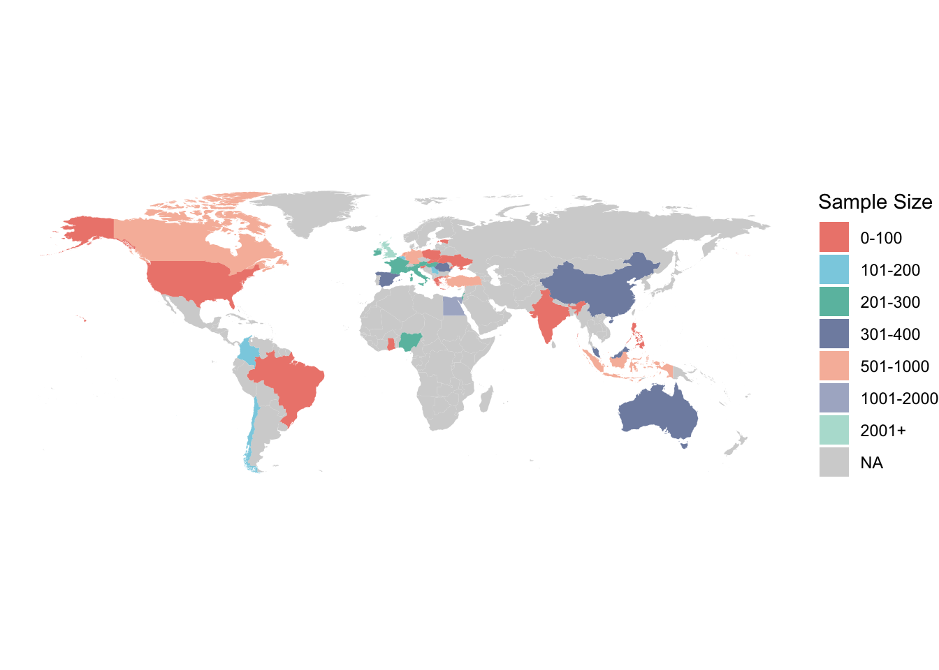
There are some NAs in the attention_amnesty column but this question was mandatory. Maybe NAs are from people who did not finish the experiment. If we keep those with progress >= 100, there will be 19.
cleaned_data %>%
  filter(progress >= 100) %>%
  miss_var_summary() %>%
  filter(variable == "attention_amnesty")
## # A tibble: 1 × 3
## variable n_miss pct_miss
## <chr> <int> <dbl>
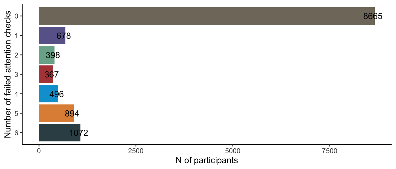
## 1 attention_amnesty 19 0.203And, let’s see how many participants will be excluded if we use any of the attention check failures and their cumulative count. For example, the cumulative_count in the second row means the number of subjects that will be removed if we exclude individuals with 6 and 5 attention check failures.
cleaned_data %>%
  count(n_att_fails) %>%
  arrange(desc(n_att_fails)) %>%
  mutate(cumulative_count = cumsum(n)) %>%
  kable() %>%
kableExtra::kable_styling()| n_att_fails | n | cumulative_count |
|---|---|---|
| 6 | 1072 | 1072 |
| 5 | 894 | 1966 |
| 4 | 496 | 2462 |
| 3 | 367 | 2829 |
| 2 | 398 | 3227 |
| 1 | 678 | 3905 |
| 0 | 8665 | 12570 |
We have decided on different criteria for excluding participants. Here is the N after applying each criterion:
cleaned_data %>% # Total N= 12570
  filter(country != "Saudi Arabia") %>% # after excluding Saudi Arabia= 12470
  filter(big >= 0 & big <= 100) %>% # excluding weird numbers. Did not change anything since we do not have the actual BiG values
  filter(n_att_fails < 4) %>% # after excluding more than 3 attention failure= 10043
  filter(attention_amnesty == "Yes") %>% # after excluding No and NAs to the honesty q = 9124
  filter(crt_cheat == "No") %>%# after excluding those admitted to searching for CRT= 8240
  count()
## # A tibble: 1 × 1
## n
## <int>
## 1 8213Two important points:
This actual number might be smaller because we have no BiG to exclude participants with weird values.
We might want to exclude languages and countries with wrong translation later.
We also might exclude countries with small N. Let’s check the N for each country after excluding participants:
excluded_data <-
  cleaned_data %>% # Total N= 12570
  filter(country != "Saudi Arabia") %>% # after excluding Saudi Arabia= 12470
  filter(big >= 0 & big <= 100) %>% # excluding weird numbers. Did not change anything since we do not have the actual BiG values
  filter(n_att_fails < 4) %>% # after excluding more than 3 attention failure= 10043
  filter(attention_amnesty == "Yes") %>% # after excluding No and NAs to the honesty q = 9124
  filter(crt_cheat == "No")

excluded_data %>%
  group_by(country) %>%
  summarise(n = n())%>%
  arrange(n) %>%
  rmarkdown::paged_table()
2.2 Proportion of correct and incorrect CRT responses
First, we check the proportion of correct, intuitive, and other (incorrect but not intuitive) CRT responses across each country. This plot can help us checking if CRT items are translated correctly for each language.
excluded_data %>%
  select(unique_id, country, crt_n_correct, crt_n_intuitive, crt_n_other) %>%
  pivot_longer(c(crt_n_correct, crt_n_intuitive, crt_n_other), names_to = "crt_type",
               values_to = "val") %>%
  mutate(crt_type = case_match(crt_type,
                               "crt_n_correct" ~ "Correct",
                               "crt_n_intuitive" ~ "Intuitive",
                               "crt_n_other" ~ "Other")) %>%
  ggplot(aes(x = crt_type, y = val, fill = crt_type))+
  geom_bar(position = "dodge", stat = "summary", fun = "mean") +
  # geom_boxplot(outlier.color = NA )+
  facet_wrap(~country, nrow = 3) +
  theme_classic()+
  labs(x=NULL, y=NULL) +
  theme(legend.position = "none",
        axis.text.x = element_text(angle = 45, vjust = 1, hjust=1)) +
  scale_fill_manual(values = c("darkgreen", "steelblue", "chocolate3"))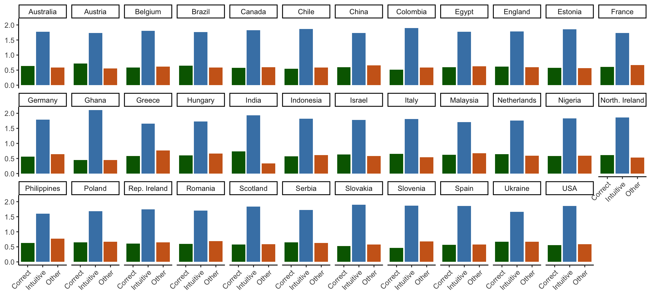
same plot but breaking than by language instead of country:
excluded_data %>%
  select(unique_id, country, crt_n_correct, crt_n_intuitive, crt_n_other) %>%
  pivot_longer(c(crt_n_correct, crt_n_intuitive, crt_n_other), names_to = "crt_type",
               values_to = "val") %>%
  mutate(crt_type = case_match(crt_type,
                               "crt_n_correct" ~ "Correct",
                               "crt_n_intuitive" ~ "Intuitive",
                               "crt_n_other" ~ "Other")) %>%
  ggplot(aes(x = crt_type, y = val, fill = crt_type))+
  geom_bar(position = "dodge", stat = "summary", fun = "mean") +
  # geom_boxplot(outlier.color = NA )+
  facet_wrap(~country, nrow = 5) +
  theme_classic()+
  labs(x=NULL, y=NULL) +
  theme(legend.position = "none",
        axis.text.x = element_text(angle = 45, vjust = 1, hjust=1)) +
  scale_fill_manual(values = c("darkgreen", "steelblue", "chocolate3"))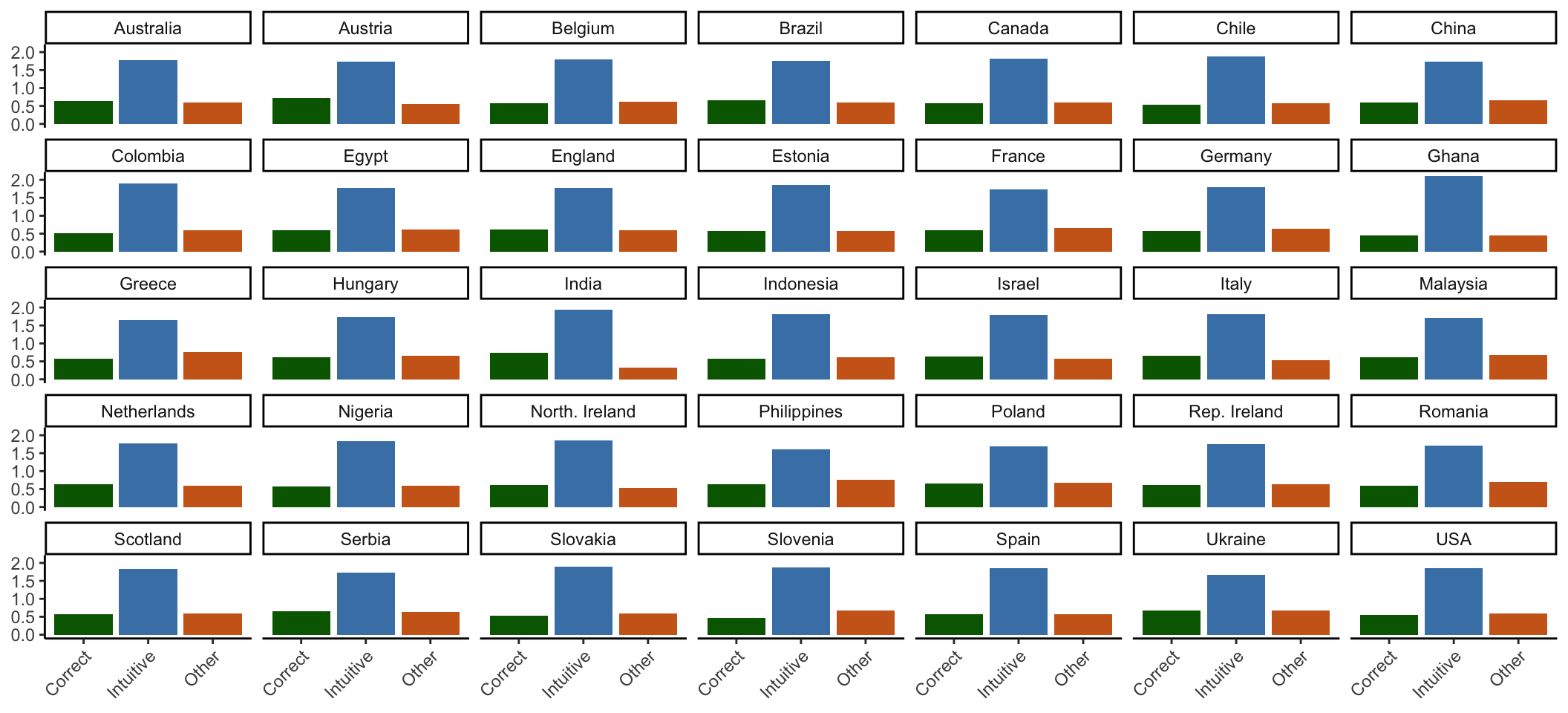
2.3 Missing values
Next, let’s see the proportion of missing values for each variable before excluding participants:
gg_miss_var(cleaned_data)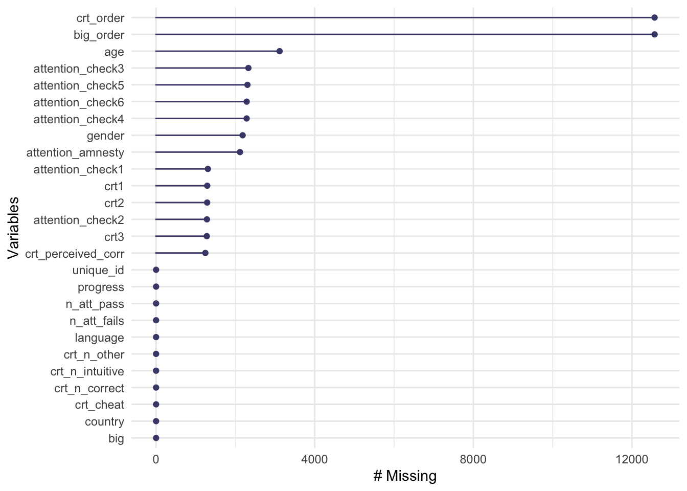
miss_var_summary(cleaned_data) %>%
  rmarkdown::paged_table()
And after excluding participants:
gg_miss_var(excluded_data)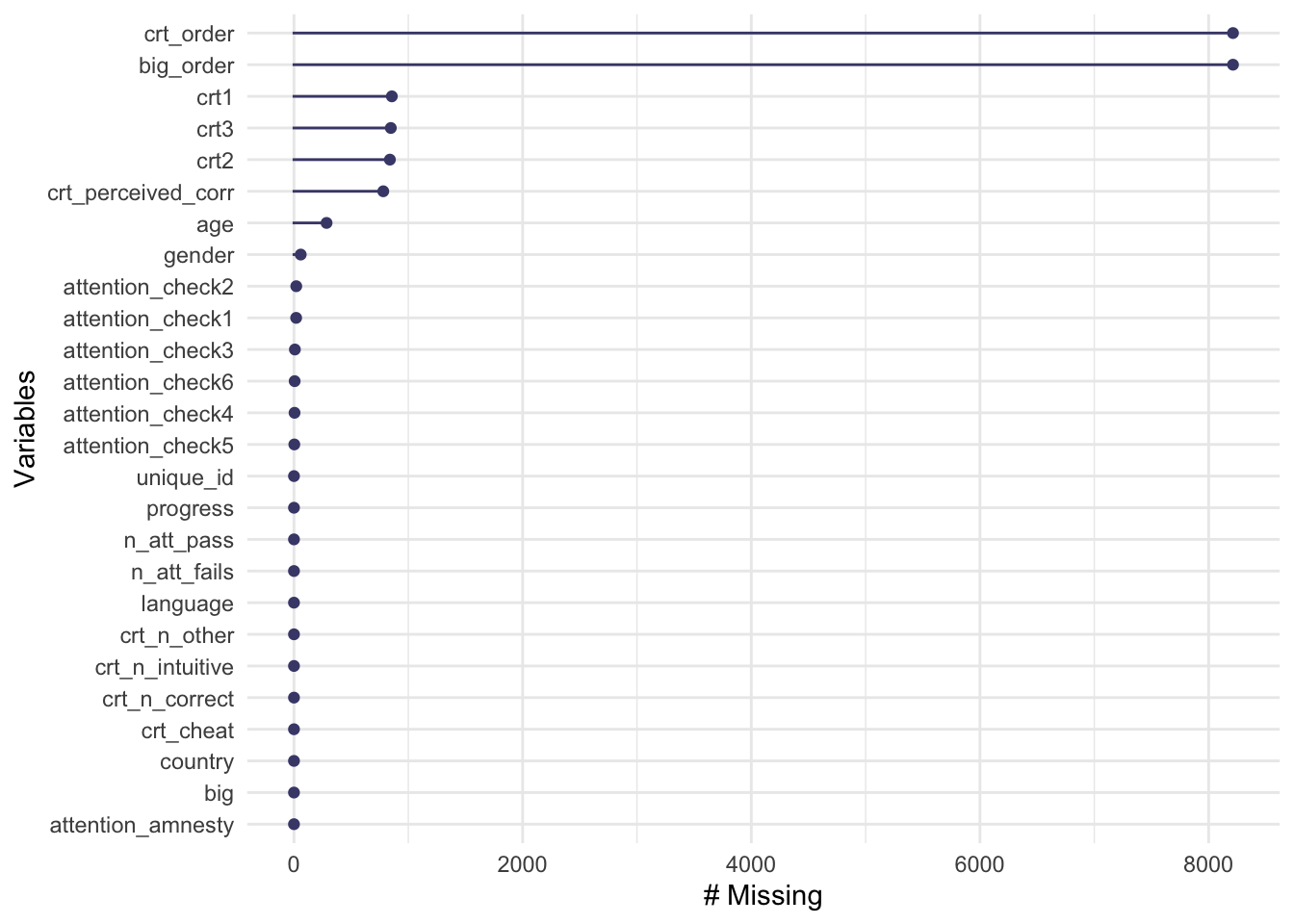
miss_var_summary(excluded_data) %>%
  rmarkdown::paged_table()
2.4 Correlation
Now, let’s check the correlation between BiG and CRT indexes (reflective/correct CRT and intuitive CRT).
(excluded_data %>%
  ggplot(aes(x = crt_n_correct, y = big))+
  geom_point(color= "steelblue", alpha = .2) +
  theme_classic()+
  facet_wrap(~"Reflective CRT") +
  geom_smooth(method='lm', color= "chocolate3", se = F)+
  labs(x="Number of correct CRT responses", y="Belief in God") +
  theme(legend.position = "none")) +
(excluded_data %>%
  ggplot(aes(x = crt_n_intuitive, y = big))+
  geom_point(color= "steelblue", alpha = .2) +
  theme_classic()+
  facet_wrap(~"Intuitive CRT") +
  geom_smooth(method='lm', color= "chocolate3", se = F)+
  labs(x="Number of intuitive CRT responses", y=NULL) +
  theme(legend.position = "none"))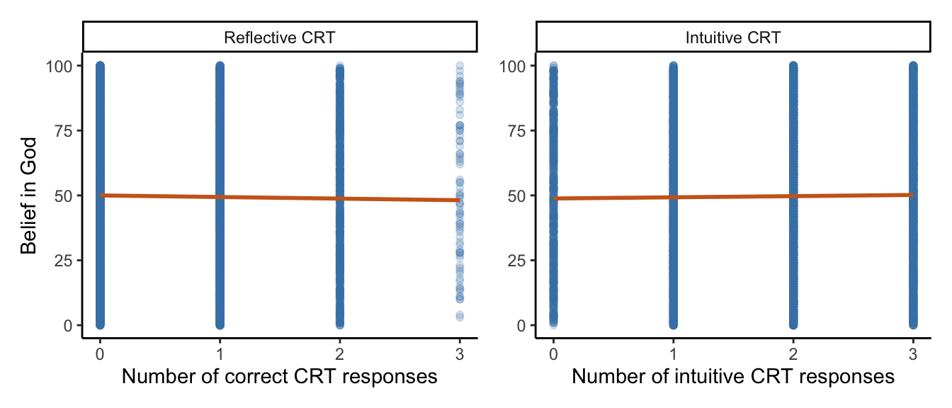
Now, let’s break down these plots by country:
excluded_data %>%
  ggplot(aes(x = crt_n_correct, y = big))+
  geom_point(color= "steelblue", alpha = .2) +
  facet_wrap(~country, nrow = 5) +
  theme_classic()+
  geom_smooth(method='lm', color= "chocolate3", se = F)+
  labs(x="Number of correct CRT responses", y="Belief in God") +
  theme(legend.position = "none")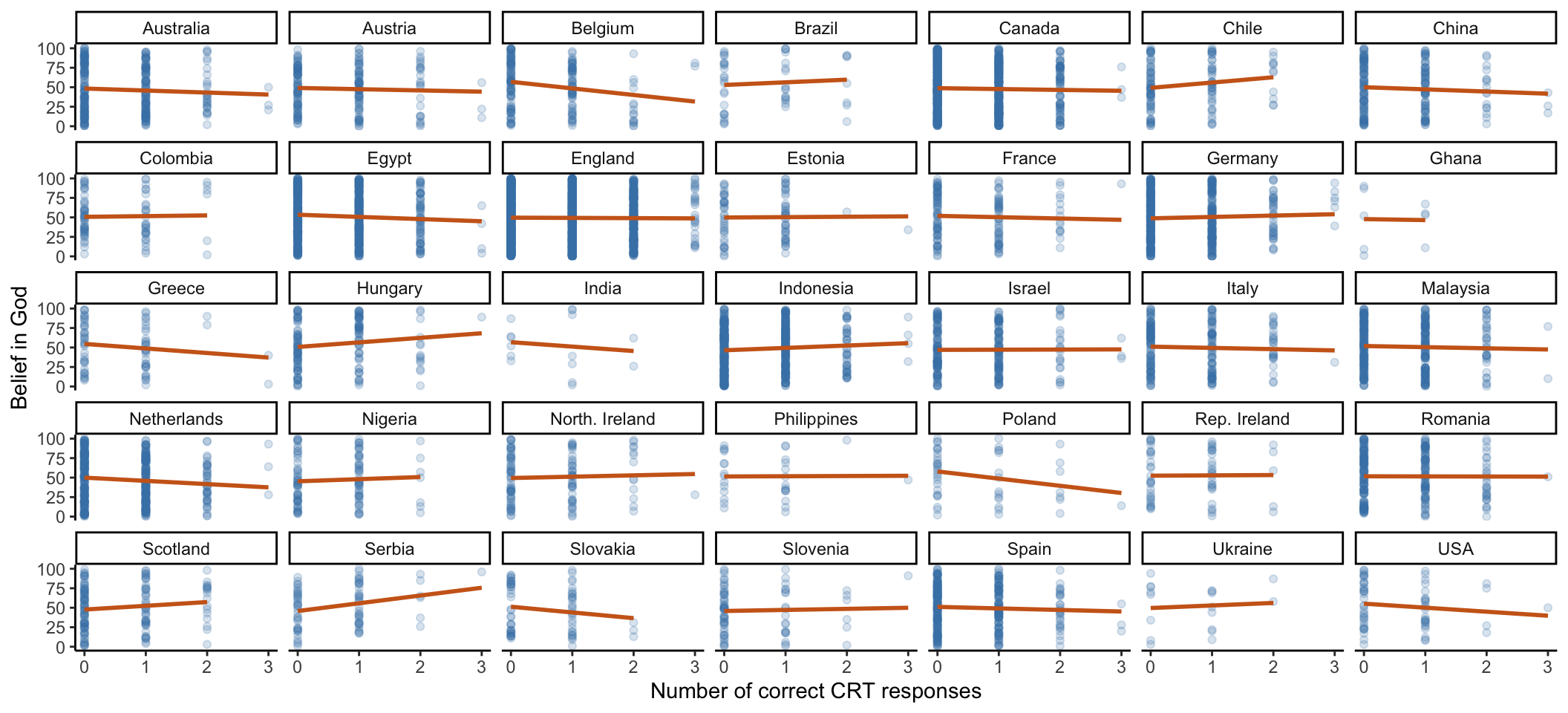
excluded_data %>%
  ggplot(aes(x = crt_n_intuitive, y = big))+
  geom_point(color= "steelblue", alpha = .2) +
  facet_wrap(~country, nrow = 5) +
  theme_classic()+
  geom_smooth(method='lm', color= "chocolate3", se = F)+
  labs(x="Number of intuitive CRT responses", y="Belief in God") +
  theme(legend.position = "none")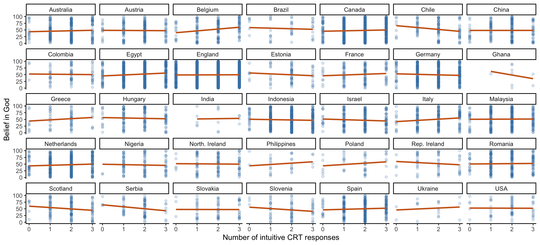
2.5 Attention check
Figure below shows the distribution of failed attention checks (i.e., how many people failed n attention checks) before excluding anyone:
cleaned_data %>%
  group_by(n_att_fails) %>%
  summarise(n = n()) %>%
  mutate(n_att_fails = fct_rev(as.factor(n_att_fails))) %>%
  ggplot(aes(x = n, y = n_att_fails, fill = n_att_fails))+
  geom_bar(position = "dodge", stat = "summary", fun = "mean") +
  theme_classic()+
  labs(y= "Number of failed attention checks", x="N of participants") +
  theme(legend.position = "none") +
  scale_fill_jama() +
  geom_text(aes(label = n), hjust = .6)