Chapter 2 Hypothesis Testing

2.1 Rock-Paper-Scissors

# This example illustrate how to find the binomial distribution of the Rock-Paper-Scissors example
numberTrial <- 12
parameter <- 1/3
probability <- function(n, x) {
    factorial(n) / factorial(n-x) / factorial(x)*(parameter)^x*(1-parameter)^(n-x)
  }
# create a dataframe for saving the probability of different number of scissors thrown out of 12 times under the null hypothesis
distvector <- vector('numeric',length = 13)
for (i in 0:12){
  distvector[i+1] <- probability(12,i)
}
dis <- as.data.frame(cbind(seq(0,12),distvector))
dis

##    V1   distvector
## 1   0 7.707347e-03
## 2   1 4.624408e-02
## 3   2 1.271712e-01
## 4   3 2.119520e-01
## 5   4 2.384460e-01
## 6   5 1.907568e-01
## 7   6 1.112748e-01
## 8   7 4.768921e-02
## 9   8 1.490288e-02
## 10  9 3.311751e-03
## 11 10 4.967626e-04
## 12 11 4.516023e-05
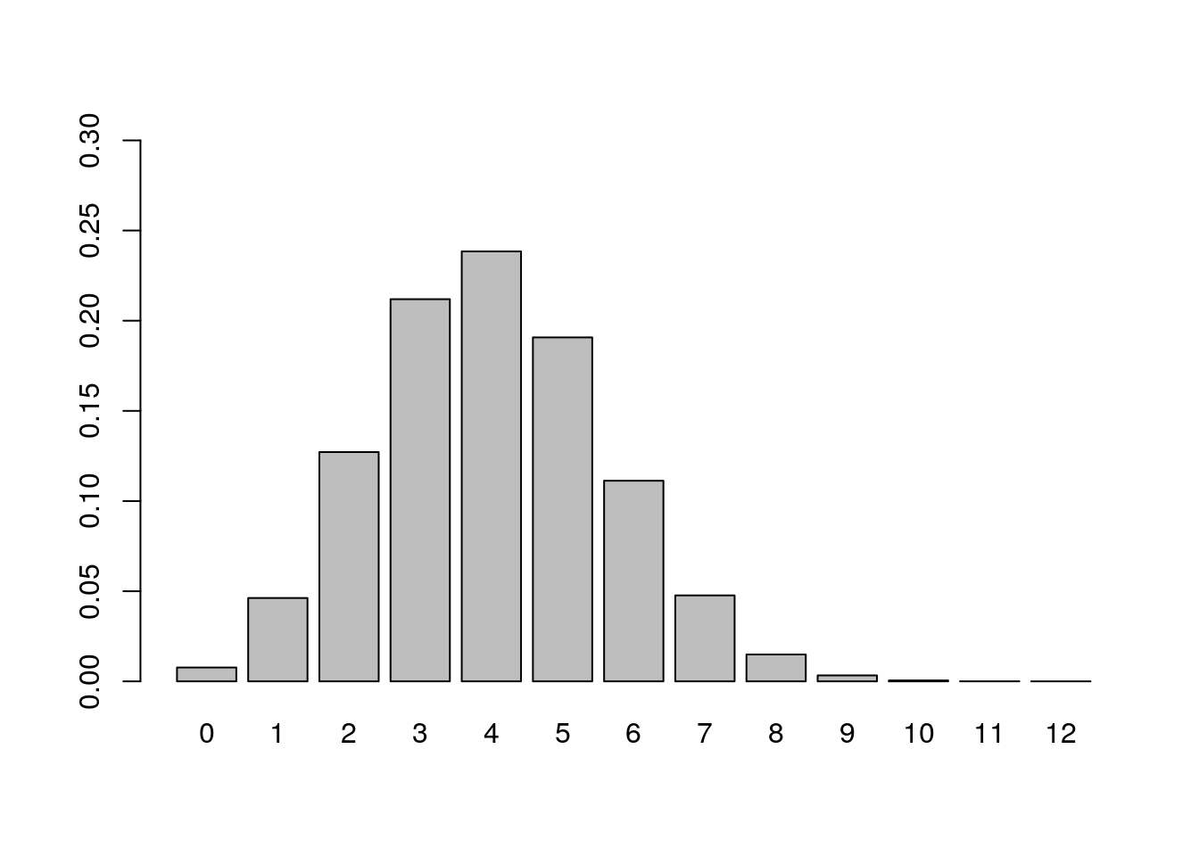
## 13 12 1.881676e-06

# Plot the distribution of throwing scissors
barplot(dis$distvector,ylim=c(0,0.3),names.arg = dis$V1)