3.2 Indexing

If your data fits in memory there is no advantage to putting it in a database: it will only be slower and more frustrating.(Hadley Wickham, RStudio, Edgar Ruiz 2019)

It can be a hassle working with databases on ad-hoc data analysis projects, but in the context of Shiny Application development, a database can help the app scale.

For example, imagine we are tasked with building a shiny dashboard to analyze New York City Yellow Taxi Trip public data located at https://on.nyc.gov/2tn71Qq. If we leave the data in a CSV format, then how does it perform compared to data imported to a database?

We can compare performance using the microbenchmark package. The following code downloads a month worth of taxi cab data and imports the file into a SQL table. I use a T-SQL bulk command because it is orders of magnitude faster at importing data then using an R function or single SQL insert statement.

url <- "https://s3.amazonaws.com/nyc-tlc/trip+data/yellow_tripdata_2018-01.csv"
download.file(url,"D:/Cab_Data/yellow_tripdata_2018-01.csv")

packages <- list('odbc','DBI','tidyverse','microbenchmark')
aa <-lapply(packages, require, character.only = TRUE,quietly = TRUE)

con <- dbConnect(odbc(),Driver = 'SQL Server',Server = '.\\snapman'
                 , Database = 'Cab_Demo', trusted_connection = TRUE)


dbExecute(con,"CREATE TABLE [dbo].[yellow_tripdata_2018-01](
    [VendorID] [smallint] NULL,
    [tpep_pickup_datetime] [datetime] NULL,
    [tpep_dropoff_datetime] [datetime] NULL,
    [passenger_count] [smallint] NULL,
    [trip_distance] [real] NULL,
    [RatecodeID] [smallint] NULL,
    [store_and_fwd_flag] [varchar](1) NULL,
    [PULocationID] [smallint] NULL,
    [DOLocationID] [smallint] NULL,
    [payment_type] [smallint] NULL,
    [fare_amount] [real] NULL,
    [extra] [real] NULL,
    [mta_tax] [real] NULL,
    [tip_amount] [real] NULL,
    [tolls_amount] [real] NULL,
    [improvement_surcharge] [real] NULL,
    [total_amount ] [real] NULL
) ON [PRIMARY]")

dbExecute(con,"BULK INSERT [dbo].[yellow_tripdata_2018-01]
FROM 'D:\Cab_Data\yellow_tripdata_2018-01.csv'
WITH (FORMAT = 'CSV')"

With the data loaded, we can run a simulate a sample workload. The following dplyr queries perform a filter and count of the rows. One query is pointed at the CSV and the other at the SQL table.

fs <- function() csvquery <- trips_fs %>% 
    filter(tpep_dropoff_datetime >= '2018-01-02 07:28:00'
          ,tpep_dropoff_datetime <= '2018-01-02 07:30:00') %>%
    summarise(pcount= n())
  rs<- suppressMessages(compute(csvquery))

db <- function() sqltable <- trips_db %>% 
    filter(tpep_dropoff_datetime >= '01-02-2018 13:28'
           ,tpep_dropoff_datetime <= '01/02/2018 13:30')  %>%
    summarise(pcount= n())
  rs1<-suppressMessages(compute(sqltable))

The benchmark function reveals a performance difference between the choice of storage. The CSV query had a lower median execution time. Thus, it would seem the claim that putting data in the database would make the analysis run slower is vindicated.

rs<-microbenchmark(db(),fs(),times = 100)
rs<-as.data.frame(rs)
rs$time <- rs$time/1000000
rs <- rs %>% filter(time < 1000) # Remove outliers on upp
ggplot(rs, aes(x=expr, y=time, fill=expr)) +
 geom_boxplot(alpha=0.4) +
    theme(text = element_text(size=20))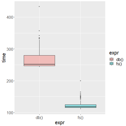

But the story changes when we add an index to the table.

ms<-dbExecute(con,
'CREATE NONCLUSTERED INDEX nc_yellow_trip
 ON [yellow_tripdata_2018-01](tpep_dropoff_datetime)'
 )

The function pointed at the SQL table now outperforms the CSV function.

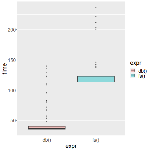
The db() function works faster because the query uses the index to seek into the data. Without an index, the query had no choice but to scan every single data page to satisfy the filter condition.

Indexing a table is a bit of art and a bit of science. Creating the best index can be challenging even for veteran DBAs. Columns used for filtering, like the query in the workload above, make good candidates for an index. Imagine you need to look up information about George Washington in a history textbook. There are two physical ways to execute this query: 1) Read the contents of all the pages or 2) Go to the index in the back of the book and read just the pages associated with George Washington. The second method seeks the relevant pages and takes far less time than reading through all the pages. A SQL index based on a filtering column is roughly analogous to the book example.

References

Hadley Wickham, RStudio, Edgar Ruiz. 2019. “Dbplyr: A Dplyr Back End for Databases.” https://CRAN.R-project.org/package=dbplyr.