Chapter 2 Linear Regression by OLS and MLE
2.1 OLS
In this first chapter we will dive a bit deeper into the methods outlined in the video "What is Maximum Likelihood Estimation (w/Regression). In the video, we touched on one method of linear regression, Least Squares Regression. Recall the general intuition is that we want to minimize the distance each point is from the line. In other words, we want to minimize the residual.
INSERT GIF OF RESIDUAL FIT FROM VIDEO
You already have a basic intuition for how this works, but let’s see how to employ least squares using some basic programming. We will use data on nest temperature and birth weight tp put these intutions into practice.
Under the hood I have generated some toy data to analyze, rather than using the standard mtcars or iris datasets (as fun as they are)
2.1.1 The data
In this dataset, julian describes the day of the year hatchlings were born, nest_temp describes the temperature of the nest throughout incubation, and birth_weight describes the average mass of a hatchling in grams.
##      julian nest_temp birth_weight
## 1 105.37724  26.90120     53.51261
## 2  91.44068  29.85848     52.49336
## 3 111.25589  25.15303     52.46664
## 4  80.24140  31.77687     51.79504
## 5 105.32226  35.71426     52.38861
## 6 108.98875  36.87243     53.32003
Let’s say we want to see if there is a relationship between an julian date and birth weight. We are going to plot date on the \(x\) axis and weight on the \(y\) axis.
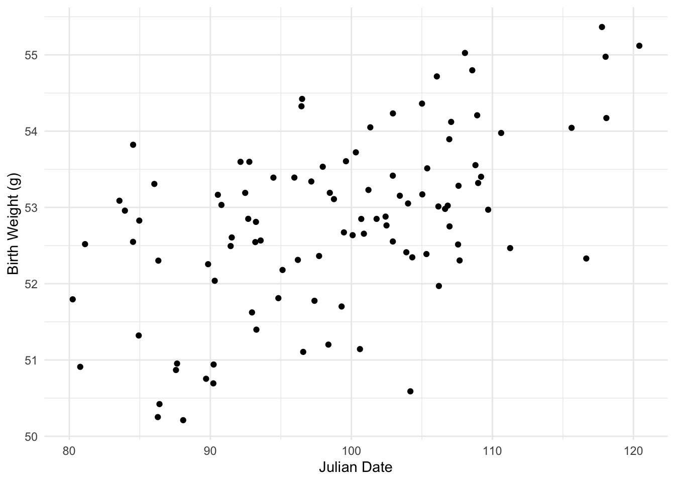
There seems to be a significant positive trend between julian date and birth weight. Recall from the video your basic intuation for fitting a line of best fit between these data is to find the line that minimizies the residual distances for each observation. To start, let’s fit a few different possible lines to the data and see how well each line fits the data under the least squares method. Eye-balling the plot I would fit a line with \(y\)-intercept about \(43\) (I played around with this a bit) and slope of (looks like a rise of 2 and run of 20) so \(.1\)? That sounds mildly reasonable I think.
Let’s also fit a line with 0 slope and intercept at whatever the mean of our y value is (in this case 52.8).
ggplot(birth_data, aes(julian, birth_weight)) + geom_point() + xlab("Julian Date") +
  geom_abline(slope = .1, intercept = 43, colour = "blue") +
  geom_abline(slope = 0, intercept = mean(birth_data$birth_weight), colour = "red") +
  theme_light()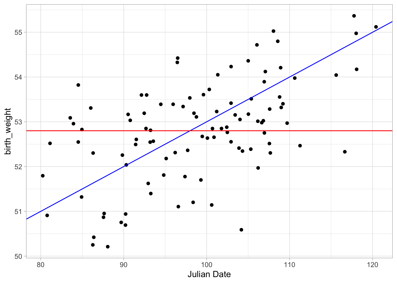
So let’s look at the residuals for our first line. Let’s make a new dataframe to calculate residuals for both of our lines
x = birth_data$julian
y = birth_data$birth_weight
y1 = (x*0.1) + 43 #line 1
y1_resid = y1-y #caluclate residual for line 1
y2 = (x*0) + mean(birth_data$birth_weight) #line 2
y2_resid = y2-y #caluclate residual for line 2
data = cbind.data.frame(x,y,y1,y1_resid,y2,y2_resid)
Now we can visualize these resdidual distances
ggplot(data, aes(x, y)) + geom_point() + xlab("Julian Date") +
  geom_abline(slope = .1, intercept = 43, colour = "blue") +
  geom_segment(xend = x, yend = y1, linetype = "dotted") + #add residuals
  theme_light()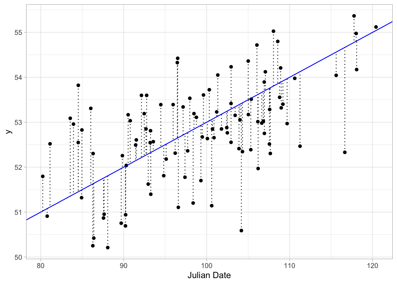
2.1.2 The math
Remember, for least squares, our goal is to minimize the total sum of the squares of the residuals.
\[ \sum_i^n = (y_i - \beta_0 + \beta_1x_1)^2 \]
So, lets see what this sum of squares is for our first line. Simple enough.
## [1] 101.7855So, what is the sum of the squared residuals for the flat line.
ggplot(data, aes(x, y)) + geom_point() + xlab("Julian Date") +
  geom_abline(slope = 0, intercept = mean(birth_data$birth_weight), colour = "red") +
  geom_segment(xend = x, yend = y2, linetype = "dotted") + #add residuals
  theme_light()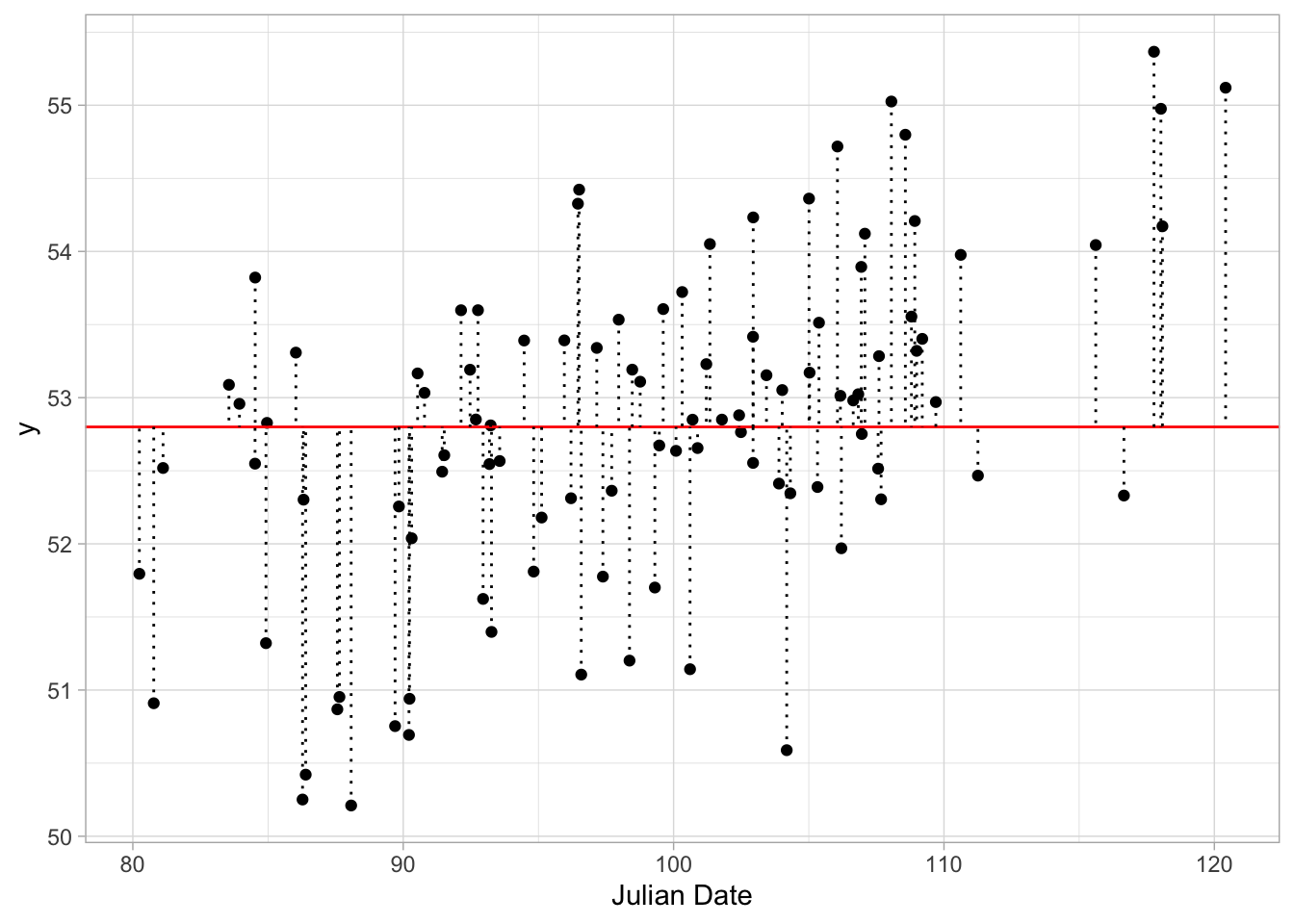
## [1] 128.2292So the total sum of squares is higher for the second line, indicating a worse fit to the data.
This is great, but not surprising. We intentionally chose a relatively good and a relatively bad fiting line. So, how could we define a function that can test any given slope and intercept and determine the value that minimizes the sum of the squared residuals. We can take advantage of some of R’s built in functionality to use what we know about least squares to minimize the equation of our line:
\[ y_i = \beta_0 + \beta_1x_i \]
Again, our residuals can then be difend simply as
\[ y_i - \beta_0 - \beta_1x_i \] and our sum of the squared residuals as
\[ \sum_i^n (y_i - \beta_0 - \beta_1x_i)^2 \]
So, now we know our goal is to minimize this function. How to we do that? R has a nice built in optimization function that can solve this for us. So, what we will do is define our function (sum of the squared residuals) then tell R to optimize that function.
First, we will make a function that takes as input our observed y values and calculates a residual based on some proposed slope and intercept parameter values.
leastsq <- function(par, y){ #inputs are parameters to be estimated and y values
  sum((y - par[1] - par[2]*x)^2) #par[1] will be intercept; par[2] will be slope
 #imagine this reads:
 #sum(y - B_0 - B_1*x_i)^2
 #we will then input our parameter values when we want to run the function down below
}
We the use R’s built in optim() function to find which values minimze our defined function.
We are optimizing both the intercept, which we have defined as our first parameter (\(\beta_0\)) and slope as our second parameter (\(\beta_1\))
OLS <- optim(
  c(int = 1, slope = 0), #^inputting (and naming) our parameter values
  #We choose starting values for the algorithm to start at
  #You can play aorund with different starting values to see if the algorithm always finds the same minimum
  fn = leastsq, #function to optimize
  y = birth_data$birth_weight) #y values

round(OLS$par, 3)
## int slope
## 46.247 0.0662.1.3 A tangent on optimizers
I want to just give a visual intution for what we are doing here. I am as of yet unsure if this explanation will end up in the video so I am including a little written sidebar here. Effectively, all regression problems (and many many other statistical and machine learning problems) boil down to finding the minimum or maximum of a function. You are iterating across all possible values and finiding where the fucntion is minimized. Where statistical pakcages often differ from one another is in the optimizers they use or the heuristics they use to choose an optimizer. For our problem, we want to iterate across every slope and intercept to see which combination gives us the minimal sum of squared residuals.Analytically this isnt horribly difficult. We just need to create a combination of every slope and intercept and calulcate the residual.
So for our data lets just say we wanted to determine the residual for every possible slope and intercept (or at least a big range of values)
I’ll use our guess of 0.1 and 43 to generate a range of possibilities
possible_m = seq(-0.1,0.3, 0.016)
possible_b = seq(35, 55, 0.4)
df = expand.grid(possible_m, possible_b) %>% rename(m = Var1, b = Var2)So now what I am going to do is calculate the total residuals for every combination of slope and intercept given our observed x and y values
for(i in 1:nrow(df)){
x = pull(birth_data, julian)
y = pull(birth_data, birth_weight)
y1 = (x*df$m[i]) + df$b[i]
df$resid[i] = sum((y1 - y)^2)
}So now that we have our squared residual for every slope and intercept combination, we can plot that as a 3-dimensional surface
So this is the function we are minimizing.For very simple models, these functions are easy to optimize. There is a clear valley to our parameter space and you can imagine it would be fairly simple to arrive at a minimum of this function. For complex models this isnt always the case. You might imagine a wiggly surface with multiple local minima or a surface where there just isnt a very clear valley. Where many statistical test “fail” or why many error messages exist is because this function can’t effectively be optimized. For example, convergence errors, boundary errors, etc all refer to issues in how the algorithm arrives at a minima. This will be covered in detail in a future video because I think its really fun (Hence this weird tangent).
Another correlated tangent: you can play around with this function to see how different optimization functions behave. Many different algorithms exist and it is important to understand how each behaves. For example, the deafult optimizer for the lmer() function in R is the “bobyqa” optimizer. Often when you run into convergence errors with lmer this can be hurdled by specifying a different optimizer function, such as optimx or Nelder-Mead. glm and lmer also let you test multiple optimizers on your model to see ow they behave. Here is a list of all the optimizer algorithms that can be used (these are roughly the same ones that use used in
lmandlmer)
method = c("Nelder-Mead", "BFGS","CG", "L-BFGS-B", "SANN") #Brent is only used for one-dimensional problems so I am excluding it
preds = list()
pars = list()
for(i in 1:length(method)){
preds[[i]] = optim(c(int = 1, slope = 0), fn = leastsq, y = birth_data$birth_weight, method = method[i])
pars[[i]] = round(preds[[i]]$par,3)
}
names(pars) = methodLet’s play a game. Which optimization methods are least like the others?*
## $`Nelder-Mead`
##    int  slope
## 46.247  0.066
##
## $BFGS
## int slope
## 46.286 0.066
##
## $CG
## int slope
## 15.770 0.372
##
## $`L-BFGS-B`
## int slope
## 46.286 0.066
##
## $SANN
## int slope
## 11.694 0.413
CGandSANNrequire some user inputs to work optimally. They are best for large, complex optimization problems and so are less ideal for general-purpose. The authors of these packages choose optimization algorithms that maximize both convergence and speed as defaults.
2.2 Back to the main stuff
##    int  slope
## 46.247  0.066
So, our defined function has found that the slope and intercept that minimize the sum of the squared residuals are \(int = 46.247\) and \(slope = 0.066\). Which is asotnishingly close to our guess of \(45\) and \(0.1\)! (Admittedly I did simulate the parameter values…)
Fitting that line to the data, we get
ggplot(birth_data, aes(julian, birth_weight)) + geom_point() + xlab("Julian Date") +
  geom_abline(slope = OLS$par[2], intercept = OLS$par[1], colour = "purple")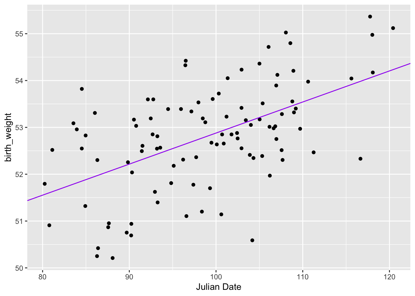
So, let’s compare this to what a common built in function might find for us. A common tool for calulating regression coefficients using least squares is the lm() function. Let’s see what we get:
## (Intercept)      julian
## 46.28632464  0.06588573
You can see we get roughly equivalent results! As a fun sanity check, here are the simulated parameter values:
## [1] "beta0 = 46.907"## [1] "beta1 = 0.0745"2.3 Multiple Parameters
So what if we have a model where we are interested in multiple parameter’s effects on a given output?
What if we were interested in how both horsepower AND engine displacement influence mpg? Well our model would then be:
mpg ~ hp + disp
Remember, our original linear model was defined as
\[ E[y] = \beta_0 + \beta_1x_i \] Recall from the video, this just means that our vector of predicted y values is given by our vector of x values, multiplied by our slope parameter (plus the intercept parameter):
\[ \begin {bmatrix} y_1 \\ y_2 \\ \vdots \\ y_n \end {bmatrix} = \beta_0 + \begin{bmatrix} x_1 \\ x_2 \\ \vdots \\ x_n \end{bmatrix} \begin{bmatrix} \beta_1 \end{bmatrix} \] Which corresponds to a system of linear equations:
\[ E[y_1] = \beta_0 + x_1\beta_1 \\ E[y_2] = \beta_0 + x_2\beta_1 \\ \vdots \\ E[y_n] = \beta_0 + x_n\beta_1 \] If we want to extend this model to include multiple parameters, we are including a new vector of \(x\) values, and a new \(\beta\) parameter. So, our new model becomes
\[ E[y_i] = \beta_0 + \beta_1x_1 + \beta_2x_2 \]
In matrix form, this model can be simplified as
\[ E[y] = \beta\textbf{X} \]
Where \(\beta\) is now a vector of all of our parameters we care about estimating and \(\textbf{X}\) is now a matrix consisting of two vectors of our predictors.
\[ E \begin {bmatrix} y_1 \\ y_2 \\ \vdots \\ y_n \end {bmatrix} = \begin{bmatrix} 1 & x_{11} & x_{21} \\ 1 & x_{12} & x_{22} \\ \vdots & \vdots & \vdots \\ 1 & x_{1n} & x_{2n} \end{bmatrix} \begin{bmatrix} \beta_0 \\ \beta_1 \\ \beta_2 \end{bmatrix} \] >Note that the column of 1s are there to indicate a constant for the \(\beta_0\) (intercept) parameter.
This corresponds to a new system of linear equations:
\[ E[y_1] = \beta_0 + \beta_1x_{11} + \beta_2x_{21} \\ E[y_2] = \beta_0 + \beta_1x_{12} + \beta_2x_{22} \\ \vdots \\ E[y_n] = \beta_0 + \beta_1x_{1n} + \beta_2x_{2n} \]
DERIVATIONS ARE COMING
If you have experience with linear algebra you have likely seen the derivation for the following equations. If you do not have experience with linear algebra, you probably don’t care. So, I will show the derivation, with minimal explanation. We will start with our basic system of linear equations.
\[ y = \textbf{X}\beta + \epsilon \]
\[ \epsilon = y- \textbf{X} \hat{\beta} \]
The sum of squared reisiduals is defined as
\[ \sum \epsilon_i^2 = [\epsilon_1,\epsilon_2,...\epsilon_n] \begin {bmatrix} \epsilon_1 \\ \epsilon_2 \\ \vdots \\ \epsilon_n \end {bmatrix} = \epsilon'\epsilon \]
Recallying that
\[ \epsilon = y - \textbf{X}\hat\beta \]
\[ \epsilon'\epsilon = (y-\textbf{X}\beta)'(y-\textbf{X}\beta) \]
Using these linear algebra terms, the least-squares parameter estimates are the vectors that minimize the function:
\[ \sum_{i=1}^n = (y-\textbf{X}\beta)'(y-\textbf{X}\beta) \]
From FOIL…
\[
\sum_{i=1}^n = y'y - 2\beta'\textbf{X}'y + \beta'\textbf{X}'\textbf{X}\beta
\]
Okay, we have derived the least squares estimators for multple regression. Now let’s see if we can use our previous leastsq function to optimize.
It’s a good idea to remind ourselves that we aren’t just palying around with symbols for fun, these equations represent the model we are trying to apply to our data:
birth_weight ~ julian + nest_temp
So, what does this model look like for our data? First, let’s construct a model matrix, which is a matrix of our x predictors with 1’s for the intercept vector.
This matrix corresponds to \(\textbf{X}\) in our system of linear equations
x = birth_data$julian
x_1 = birth_data$nest_temp
y = birth_data$birth_weight
X = model.matrix(y ~ x + x_1)
head(X)
## (Intercept) x x_1
## 1 1 105.37724 26.90120
## 2 1 91.44068 29.85848
## 3 1 111.25589 25.15303
## 4 1 80.24140 31.77687
## 5 1 105.32226 35.71426
## 6 1 108.98875 36.87243Now, we plug in the functions we derived above into our least squares function, and use par[1:3] to represent our vector of beta’s.
Note: %*% represents matrix multiplication
leastsq <- function(par, y){
  sum((t(y - X %*% par[1:3]) %*% (y - X %*% par[1:3]))^2)
  #note: t() represents the transposition
}

OLS <- optim(c(int = 1, julian = 0, nest_temp = 0), fn = leastsq,
     y = birth_data$birth_weight, method = "BFGS")
#Note: I choose to use the BFGS optimizer here.
(OLS_1 <- round(OLS$par,3))
## int julian nest_temp
## 48.090 0.066 -0.063And now let’s just double check that FOIL’ing our function above gives the same result.
leastsq <- function(par, y){
  sum((t(y)%*%y - 2%*%t(par[1:3])%*%t(X)%*%y + t(par[1:3])%*%t(X)%*%X%*%par[1:3])^2)
}


OLS <- optim(c(int = 1, julian = 0, nest_temp = 0), fn = leastsq,
     y = birth_data$birth_weight, method = "BFGS")

(OLS_2 <- round(OLS$par,3))
## int julian nest_temp
## 48.090 0.066 -0.063Now, lets see how some of R’s built-in functions can solve this problem for us. First, Using linear algebra notation, R has a convenient function called solve() which…get this…solves linear systems of equations. For us, our linear system of equations is
\[ (X'X)^{-1}X'y \]
So let’s use solve to…solve it.
##      (Intercept)      x     x_1
## [1,]     48.0903 0.0665 -0.0627
And finally, let’s see if all of our analytical techniques give similar resutls to those acquired through the ever-so-simple lm() function:
## (Intercept)      julian   nest_temp
## 48.090 0.066 -0.063## int julian nest_temp
## OLS_1 48.09000 0.06600000 -0.0630000
## 48.09030 0.06650000 -0.0627000
## 48.09032 0.06649805 -0.0627491Hoozah! We now have seen how least squares works. Now we can see how it compares and constrasts with maximum likelihood.