Chapter 6 Bayesian Inference
Bayesian inference estimates the probability, \(\theta\), that an hypothesis is true. It differs from frequentist inference in its insistence that all uncertainties be described by probabilities. Bayesian inference updates the prior probability distribution in light of new information.
Bayesian inference builds on Bayes’ Law, so let’s start there.
6.1 Bayes’ Law
Bayes’ Law is a clever re-ordering of the relationship between joint probability and conditional probability, \(P(\theta D) = P(\theta|D)P(D) = P(D|\theta)P(\theta)\), into
\[P(\theta|D) = \frac{P(D|\theta)P(\theta)}{P(D)}.\]
\(P(\theta)\) is the strength of your belief in \(\theta\) prior to considering the data \(D\).
\(P(D|\theta)\) is the likelihood of observing \(D\) from a generative model with parameter \(\theta\). Note that likelihood is the probability density, and is not quite the same as probability. For a continuous variable, likelihoods can sum to greater than 1. E.g., *
dbinom(seq(1, 100, 1), 100, .5)sums to 1, butdnorm(seq(0,50,.001), 10, 10)sums to 841.\(P(D)\) is the likelihood of observing \(D\) from any prior. It is the marginal distribution, or prior predictive distribution of \(D\). The likelihood divided by the marginal distribution is the proportional adjustment made to the prior in light of the data.
\(P(\theta|D)\) is the strength of your belief in \(\theta\) posterior to considering \(D\).
Bayes’ Law is useful for evaluating medical tests. A test’s sensitivity is its probability of observing positive test result \(D\) when medical condition \(\theta\) exists. The numerator of Bayes’ Law, the joint probability of \(D\) and \(\theta\), \(P(D \theta)\), is the test sensitivity multiplied by the prior probability, \(\mathrm{sens\times prior}\). A test’s specificity is the probability of observing negative test result \(\hat{s}\) when the condition does not exist, \(\hat{\theta}\). The specificity is the compliment of a false positive test result, \(P(\hat{D} | \hat{\theta}) = 1 - P(D | \hat{\theta})\). The denominator of Bayes’ Law is the overall probability of a positive test result, \(P(D) = P(D|\theta)P(\theta) + P(D|\hat\theta)P(\hat\theta)\) or in terms of sensitivity and specificity, \(P(D) = \mathrm{(sens \times prior) + (1 - spec)(1 - prior)}\).
Example. Suppose E. Coli is typically present in 4.5% of samples, and an E. Coli screen has a sensitivity of 0.95 and a specificity of 0.99. Given a positive test result, what is the probability that E. Coli is actually present?
\[P(\theta|D) = \frac{.95\cdot .045}{.95\cdot .045 + (1 - .99)(1 - .045)} = \frac{.04275}{.04275 + .00955} = \frac{.04275}{.05230} = 81.7\%.\]
The Bayes’ Law logic is apparent from the contingency table. The first row is the positive test result.
| E. Coli | Safe | Total | |
|---|---|---|---|
| + Test | .95 * .045 = 0.04275 | .01 * .955 = 0.00955 | 0.05230 |
| - Test | .05 * .045 = 0.00225 | .99 * .955 = 0.94545 | 0.94770 |
| Total | 0.04500 | 0.95500 | 1.00000 |
6.2 Bayesian Inference
Bayesian inference extends the logic of Bayes’ Law by replacing the prior probability estimate that \(\theta\) is true with a prior probability distribution that \(\theta\) is true. Rather than saying, “I am x% certain \(\theta\) is true,” you are saying “I believe the probability that \(\theta\) is true is somewhere in a range that has maximum likelihood at x%”.
Let \(\Pi(\theta)\) be the prior probability function of \(\theta\). \(\Pi(\theta)\) has a pmf or pdf \(P(\theta)\), and a set of conditional distributions called the generative model for the observed data \(D\) given \(\theta\), \(\{f_\theta(D): \theta \in \Omega\}\). \(f_\theta(D)\) is the likelihood of observing \(D\) given \(\theta\). Their product, \(f_\theta(D)P(\theta)\), is a joint distribution of \((D, \theta)\).
For continuous prior distributions, the marginal distribution for \(D\), called the prior predictive distribution, is
\[m(D) = \int_\Omega f_\theta(D)P(\theta) d\theta\]
For discrete prior distributions, replace the integral with a sum, \(m(D) = \sum\nolimits_\Omega f_\theta(D) P(\theta)\). The posterior probability distribution of \(\theta\), conditioned on the observance of \(D\), is \(\Pi(\cdot|D)\). It is the joint density, \(f_\theta(D) P(\theta),\) divided by the the marginal density, \(m(D)\).
\[P(\theta | D) = \frac{f_\theta(D) P(\theta)}{m(D)}\] The numerator makes the posterior proportional to the prior. The denominator is a normalizing constant that scales the likelihood into a proper density function (whose values sum to 1).
It is helpful to look first at discrete priors, a list of competing priors to see how the observed evidence shifts the probabilities of the priors into their posterior probabilities. From there it is a straight-forward step to the more abstract case of continuous prior and posterior distributions.
6.3 Discrete Cases
Suppose you have a string of numbers \([1,1,1,1,0,0,1,1,1,0]\) (seven 1s and three 0s) produced by a Bernoulli random number generator. What parameter \(p\) was used in the Bernoulli function?1
Your best guess is \(p = 0.7\), but how confident are you? Posit eleven competing priors, \(\theta = [.0, .1, \ldots,1.0]\) with equal prior probabilities, \(P(\theta) = [1/11, \ldots]\).
Using a Bernoulli generative model, the likelihoods of observing seven 1s and three 0s are \(P(D|\theta) = \theta^7 + (1-\theta)^3.\)
likelihood <- theta^7 * (1 - theta)^3

data.frame(theta, likelihood) %>%
  ggplot() +
  geom_segment(aes(x = theta, xend = theta, y = 0, yend = likelihood),
               linetype = 2, color = "steelblue") +
  geom_point(aes(x = theta, y = likelihood), color = "steelblue", size = 3) +
  scale_x_continuous(breaks = theta) +
  theme_minimal() +
  theme(panel.grid.minor = element_blank()) +
  labs(title = expression(paste("Maximum likelihood of observing D is at ", theta, " = 0.7.")),
       x = expression(theta), y = expression(f[theta](D)))
The posterior probability is the likelihood divided by the marginal probability of observing \(D\) multiplied by the prior, \(P(\theta|D) = \frac{P(D|\theta)}{P(D)}\cdot P(\theta).\) In this case, the marginal probability is straight-forward to calculate: it is the sum-product of the priors and their associated likelihoods.
posterior <- likelihood / sum(likelihood * prior) * prior

data.frame(theta, prior, posterior) %>%
  pivot_longer(cols = c(prior, posterior), values_to = "pi") %>%
  ggplot() +
  geom_point(aes(x = theta, y = pi, color = name), size = 1) +
  geom_line(aes(x = theta, y = pi, color = name), size = 1) +
  scale_x_continuous(breaks = theta) +
  theme_minimal() +
  theme(panel.grid.minor = element_blank()) +
  labs(title = "Posterior probabilities are adjusted priors.",
       color = NULL,
       x = expression(theta), y = "P")
What would the posterior look like if we started with an educated guess on \(P(\theta)\) that more heavily weights \(\theta = 0.7\)?
prior <- c(.05, .05, .05, .05, .05, .10, .15, .20, .15, .10, .05)
likelihood <- theta^7 * (1 - theta)^3
posterior <- likelihood / sum(likelihood * prior) * prior
data.frame(theta, prior, posterior) %>%
  pivot_longer(cols = c(prior, posterior), values_to = "pi") %>%
  ggplot() +
  geom_point(aes(x = theta, y = pi, color = name), size = 1) +
  geom_line(aes(x = theta, y = pi, color = name), size = 1) +
  scale_x_continuous(breaks = theta) +
  theme_minimal() +
  theme(panel.grid.minor = element_blank()) +
  labs(title = "Smarter priors increase posterior probability at maximum.",
       color = NULL, x = expression(theta), y = "P")
What if we now employ a larger data set? To see, generate a sample of 100 \(\mathrm{Bernouli}(.7)\) observations.
s <- rbernoulli(100, p = 0.7) %>% as.numeric()
likelihood <- theta^sum(D) * (1 - theta)^(length(D)-sum(D))
posterior <- likelihood / sum(likelihood * prior) * prior
data.frame(theta, prior, posterior) %>%
  pivot_longer(cols = c(prior, posterior), values_to = "pi") %>%
  ggplot() +
  geom_point(aes(x = theta, y = pi, color = name), size = 1) +
  geom_line(aes(x = theta, y = pi, color = name), size = 1) +
  scale_x_continuous(breaks = theta) +
  theme_minimal() +
  theme(panel.grid.minor = element_blank()) +
  labs(title = "More observations tighten the posterior distribution.",
       color = NULL, x = expression(theta), y = expression(pi))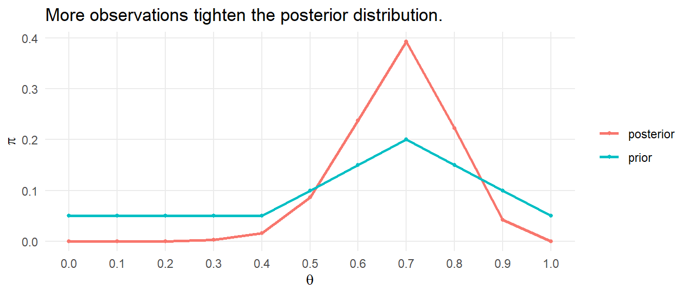
What would it look like if it also had more competing hypotheses, \(\theta \in (0, .01, .02, \ldots, 1)\).
theta <- seq(0, 1, by = .01)
prior <- rep(1/100, 101)
likelihood <- theta^sum(D) * (1 - theta)^(length(D)-sum(D))
posterior <- likelihood / sum(likelihood * prior) * prior
data.frame(theta, prior, posterior) %>%
  pivot_longer(cols = c(prior, posterior), values_to = "pi") %>%
  ggplot() +
  geom_point(aes(x = theta, y = pi, color = name), size = 1) +
  geom_line(aes(x = theta, y = pi, color = name), size = 1) +
  scale_x_continuous(breaks = seq(0, 1, by = 0.1)) +
  theme_minimal() +
  theme(panel.grid.minor = element_blank()) +
  labs(title = "More priors smooths the distribution.",
       color = NULL, x = expression(theta), y = "P")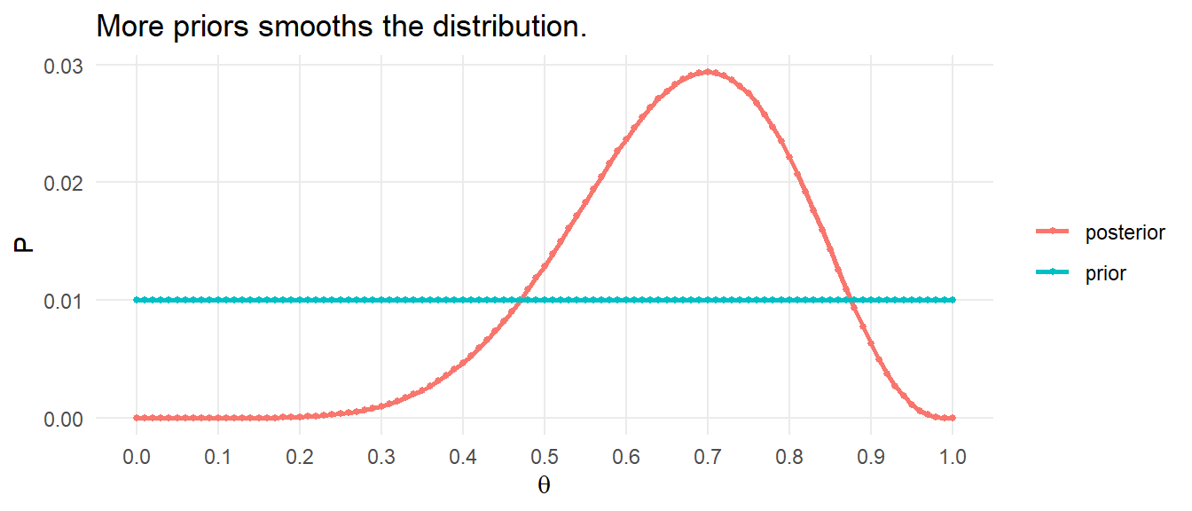
6.4 Continuous Cases
Continuing the example of inferring the parameter \(p\) used in the Bernoulli process, what if we considered all values between 0 and 1?2
When prior beliefs are best described in continuous distributions, express them using the beta, gamma, or normal distribution so that the posterior distributions are conjugates of the prior distributions with new parameter values. Otherwise, the marginal distribution is difficult to calculate. In this case, use the beta distribution, described by shape parameters, \(\alpha\) and \(\beta\).
\[P(\theta|D,\alpha,\beta) = \frac{f_\theta(D) P(\theta|\alpha,\beta)}{\int_0^1 f_\theta(D)P(\theta|\alpha, \beta)d\theta}\]
As with the discrete case, the numerator equals the likelihood of observing \(s\) if \(\theta\) is true multiplied by the prior probability, but now the prior is a \(\mathrm{Beta}(\alpha,\beta)\) distribution. The denominator is the marginal probability of \(s\).
The likelihood is
\[f_\theta(D) = \theta^a(1-\theta)^b\] where \(a\) and \(b\) are the respective counts of 1s and 0s. The prior distribution is
\[P(\theta|\alpha,\beta) = \frac{\Gamma(\alpha + \beta)}{\Gamma(\alpha)\Gamma(\beta)}\theta^{\alpha-1}(1-\theta)^{\beta-1}\]
The marginal distribution is
\[m(D|\alpha,\beta) = \frac{\Gamma(\alpha+\beta)}{\Gamma(\alpha)\Gamma(\beta)} \frac{\Gamma(\alpha+a)\Gamma(\beta+b)}{\Gamma(\alpha+a+\beta+b)}\]
Putting this all together, the posterior distribution is
\[P(\theta|s, \alpha, \beta) = \frac{\Gamma(\alpha+\beta+a+b)}{\Gamma(\alpha+a)\Gamma(\beta+b)} \theta^{\alpha-1+a}(1-\theta)^{\beta-1+b}\]
Notice the posterior equals the prior with shape parameters incremented by the observed counts, \(a\) and \(b.\)
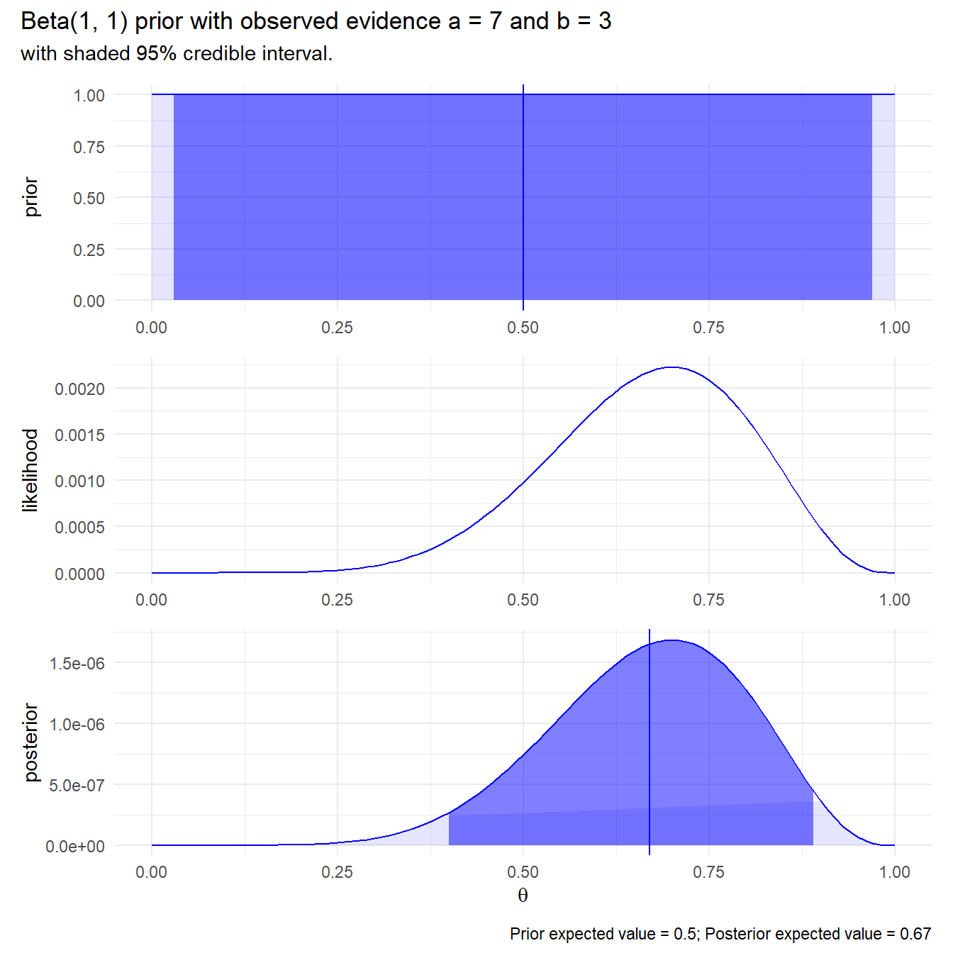
Suppose you claim complete ignorance and take a uniform \(\mathrm{Beta}(1, 1)\) prior. The posterior expected value is still pretty close!
plot_bayes <- function(alpha, beta, a, b) {

  prior_ev <- (alpha / (alpha + beta)) %>% round(2)
  posterior_ev <- ((alpha + a) / (alpha + beta + a + b)) %>% round(2)
  dat <- data.frame(theta = seq(0, 1, by = .01)) %>%
    mutate(prior = beta(alpha, beta) * theta^(alpha-1) * (1-theta)^(beta-1),
           prior_ci = theta > qbeta(.025, alpha, beta) &
                      theta < qbeta(.975, alpha, beta),
           likelihood = theta^a * (1-theta)^b,
           posterior = beta(alpha + a, beta + b) * theta^(alpha-1+a) * (1-theta)^(beta-1+b),
           posterior_ci = theta > qbeta(.025, alpha + a, beta + b) &
                      theta < qbeta(.975, alpha + a, beta + b))

  p_prior <- dat %>%
    ggplot(aes(x = theta, y = prior)) +
    geom_line(color = "blue") +
    geom_area(aes(alpha = prior_ci), fill = "blue") +
    geom_vline(xintercept = prior_ev, color = "blue") +
    scale_alpha_manual(values = c(.1, .5)) +
    theme_minimal() +
    theme(legend.position = "none") +
    labs(x = NULL)

  p_likelihood <- dat %>%
    ggplot(aes(x = theta, y = likelihood)) +
    geom_line(color = "blue") +
    theme_minimal() +
    theme(legend.position = "none") +
    labs(x = NULL)

  p_posterior <- dat %>%
    ggplot(aes(x = theta, y = posterior)) +
    geom_line(color = "blue") +
    geom_area(aes(alpha = posterior_ci), fill = "blue") +
    geom_vline(xintercept = posterior_ev, color = "blue") +
    scale_alpha_manual(values = c(.1, .5))  +
    theme_minimal() +
    theme(legend.position = "none") +
    labs(x = expression(theta))

  out <- p_prior / p_likelihood / p_posterior +
    plot_annotation(
      title = glue("Beta({alpha}, {beta}) prior with observed evidence a = {a} ",
                   "and b = {b}"),
      subtitle = "with shaded 95% credible interval.",
      caption = glue("Prior expected value = {prior_ev}; Posterior expected ",
                     "value = {posterior_ev}"))
  out
}
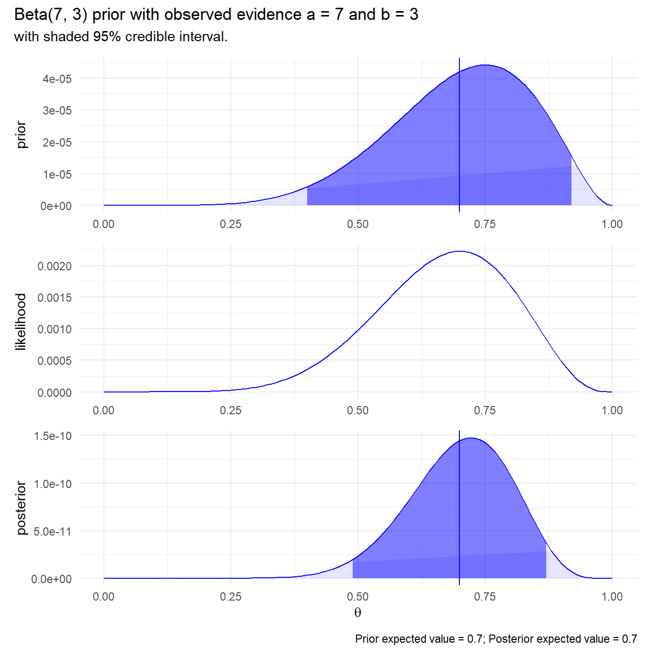
Suppose you had an inkling that \(p = 0.7\).
6.5 A Gentler Introduction
This section is my notes from DataCamp course Fundamentals of Bayesian Data Analysis in R. It is an intuitive approach to Bayesian inference.
Suppose you purchase 100 ad impressions on a web site and receive 13 clicks. How would you describe the click rate? The frequentist approach would be to construct a 95% CI around click proportion.
ad_prop_test <- prop.test(13, 100)
click_rate_mu <- ad_prop_test$estimate
click_rate_se <- sqrt(click_rate_mu*(1-click_rate_mu)) / sqrt(100)
data.frame(pi = seq(0, .30, by = .001)) %>%
  mutate(likelihood = dnorm(pi, click_rate_mu, click_rate_se),
         ci = if_else(pi >= ad_prop_test$conf.int[1] &
                        pi <= ad_prop_test$conf.int[2], "Y", "N")) %>%
  ggplot(aes(x = pi, y = likelihood)) +
  geom_line() +
  geom_area(aes(y = if_else(ci == "N", likelihood, 0)),
            fill = "firebrick", show.legend = FALSE) +
  geom_vline(xintercept = click_rate_mu, linetype = 2) +
  theme_minimal() +
  scale_x_continuous(breaks = seq(0, .3, .05)) +
  theme(panel.grid.minor = element_blank()) +
  labs(title = "Frequentist proportion test for 13 clicks in 100 impressions",
       subtitle = glue("p = {click_rate_mu}, 95%-CI (",
       "{ad_prop_test$conf.int[1] %>% scales::number(accuracy = .01)}, ",
       "{ad_prop_test$conf.int[2] %>% scales::number(accuracy = .01)})"),
       x = expression(theta))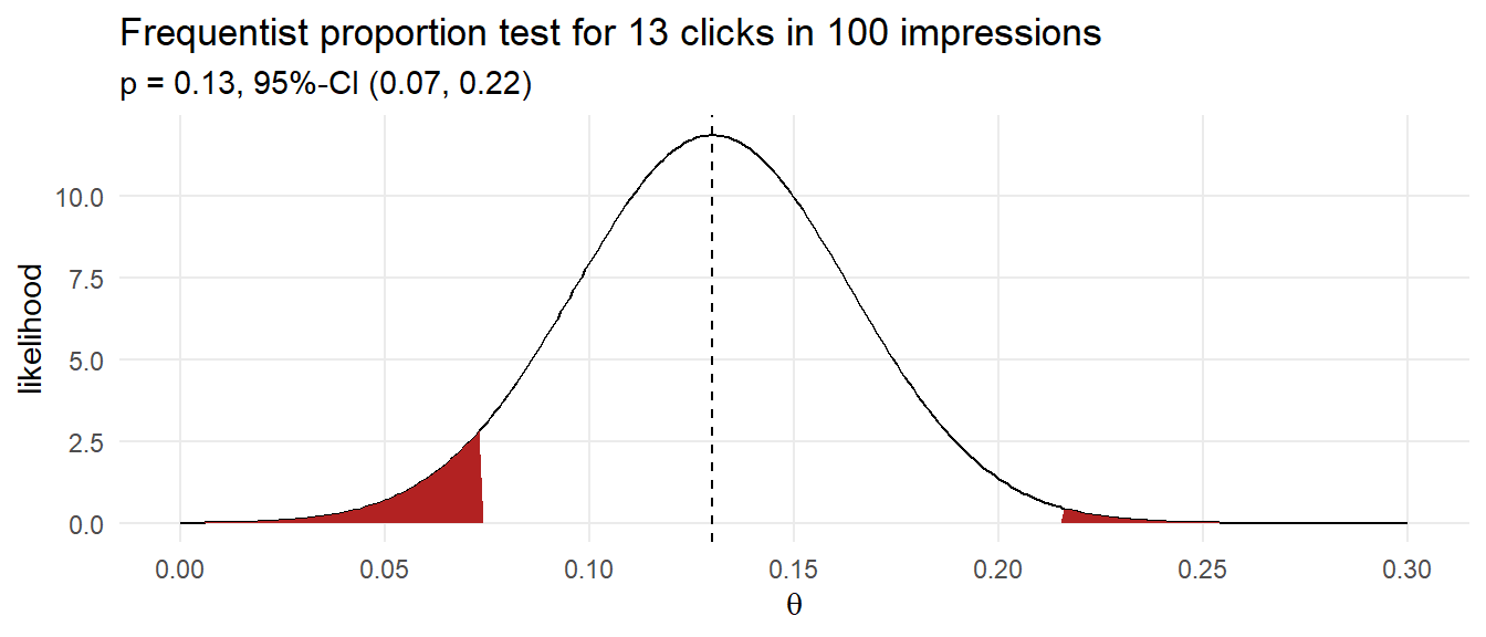
How might you model this using Bayesian reasoning? One way is to run 1,000 experiments that sample 100 ad impression events from an rbinom() generative model using a uniform prior distribution of 0-30% click probability. The resulting 1,000 row data set of click probabilities and sampled click counts forms a joint probability distribution. This method of Bayesian analysis is called rejection sampling because you sample across the whole parameter space, then condition on the observed evidence.
df_sim <- data.frame(click_prob = runif(1000, 0.0, 0.3))
df_sim$click_n <- rbinom(1000, 100, df_sim$click_prob)

df_sim %>%
  mutate(is_13 = factor(click_n == 13, levels = c(TRUE, FALSE))) %>%
  ggplot(aes(x = click_prob, y = click_n, color = is_13)) +
  geom_point(alpha = 0.3, show.legend = FALSE) +
  geom_hline(yintercept = 13, color = "red", linetype = 2) +
  theme_minimal() +
  labs(title = "Joint probability of observed clicks and click probability",
       subtitle = "with conditioning on 13 observed clicks.",
       y = "clicks per 100 ads",
       x = expression(theta))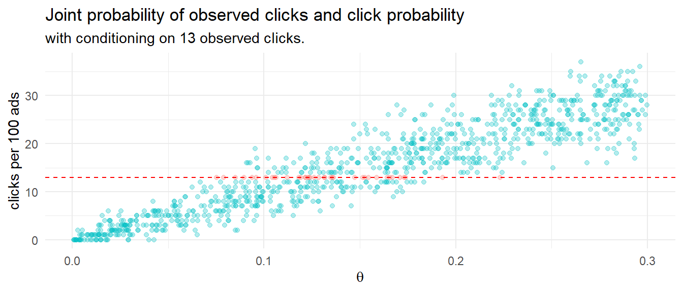
Condition the joint probability distribution on the 13 observed clicks to update your prior. The quantile() function will arrange the click probabilities that produced 13 clicks and return the .025 and .975 values - the credible interval.
# median and credible interval
sim_ci <- df_sim %>% filter(click_n == 13) %>% pull(click_prob) %>%
  quantile(c(.025, .5, .975))

df_sim %>%
  filter(click_n == 13) %>%
  ggplot(aes(x = click_prob)) +
  geom_density() +
  geom_vline(xintercept = sim_ci[2]) +
  geom_vline(xintercept = sim_ci[1], linetype = 2) +
  geom_vline(xintercept = sim_ci[3], linetype = 2) +
  scale_x_continuous(breaks = seq(0, .3, .05)) +
  theme_minimal() +
  labs(title = "Posterior click likelihood distribution",
       subtitle = glue("p = {sim_ci[2] %>% scales::number(accuracy = .01)}, 95%-CI (",
       "{sim_ci[1] %>% scales::number(accuracy = .01)}, ",
       "{sim_ci[3] %>% scales::number(accuracy = .01)})"),
       x = expression(theta), y = "density (likelihood)")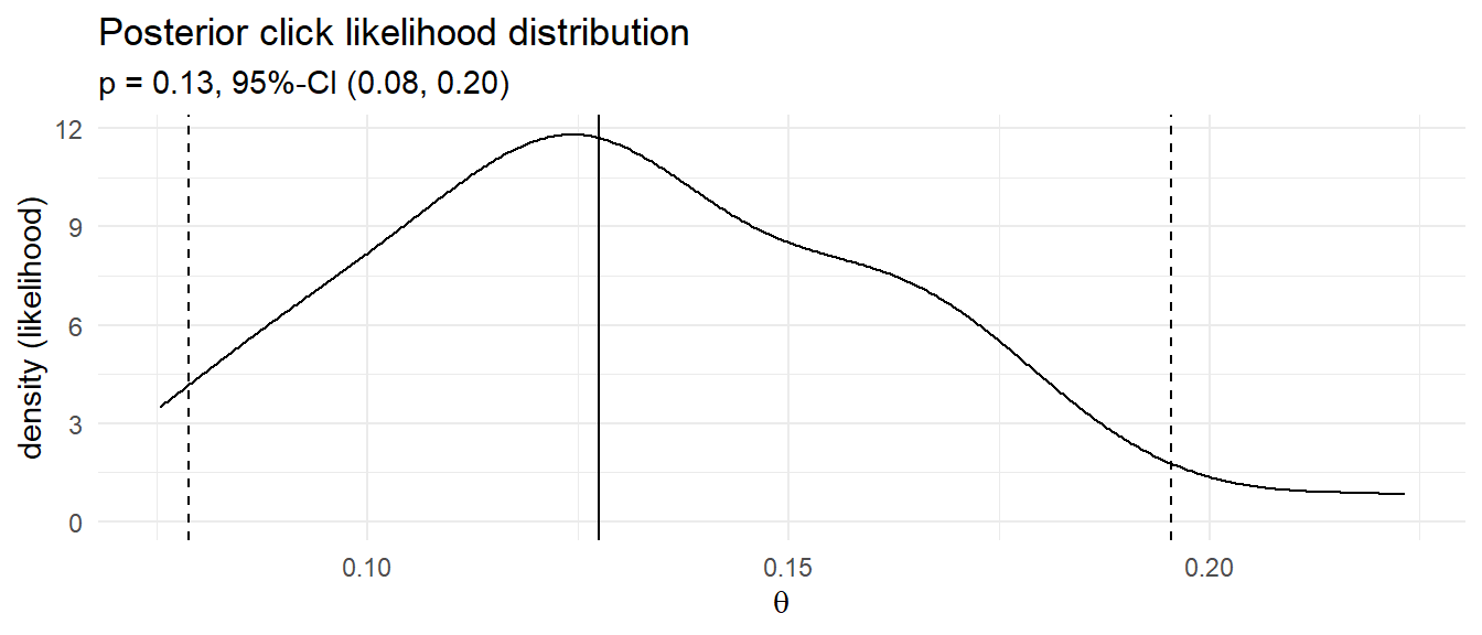
That’s pretty close to the frequentist result! Instead of running 1,000 experiments with randomly selected click probabilities and randomly selected click counts based on those probabilities, you could define a discrete set of candidate click probabilities, e.g. values between 0 and 0.3 incremented by .01, and calculate the click probability density for the 100 ad impressions. This method of Bayesian analysis is called grid approximation.
df_bayes <- expand.grid(click_prob = seq(0, .3, by = .001),
                        click_n = 0:100) %>%
  mutate(prior = dunif(click_prob, min = 0, max = 0.3),
         likelihood = dbinom(click_n, 100, click_prob),
         probability = likelihood * prior / sum(likelihood * prior))

df_bayes %>%
  mutate(is_13 = factor(click_n == 13, levels = c(TRUE, FALSE))) %>%
  filter(probability > .0001) %>%
  ggplot(aes(x = click_prob, y = click_n, color = probability)) +
  geom_point() +
  geom_hline(yintercept = 13, color = "red", linetype = 2) +
  scale_color_gradient(low = "white", high = "steelblue", guide = "colorbar") +
  theme_minimal() +
  labs(title = "Joint probability of clicks and click probability.",
       subtitle = "with conditioning on 13 observed clicks.",
       y = "clicks per 100 ads",
       x = expression(theta))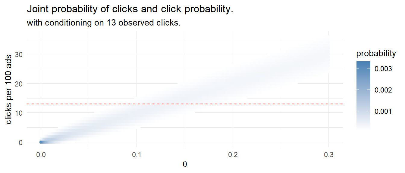
Condition the joint probability distribution on the 13 observed clicks to adjust your prior.
# median and credible interval
df_bayes_13 <- df_bayes %>% filter(click_n == 13) %>%
  mutate(posterior = probability / sum(probability))
sampling_idx <- sample(1:nrow(df_bayes_13), size = 10000, replace = TRUE, prob = df_bayes_13$posterior)
sampling_vals <- df_bayes_13[sampling_idx, ]
df_bayes_ci <- quantile(sampling_vals$click_prob, c(.025, .5, .975))

df_bayes %>%
  filter(click_n == 13) %>%
  mutate(likelihood = probability / sum(probability),
         ci = if_else(click_prob >= df_bayes_ci[1] &
                        click_prob <= df_bayes_ci[3], "Y", "N")) %>%
  ggplot(aes(x = click_prob, y = likelihood)) +
  geom_line() +
  geom_area(aes(y = if_else(ci == "N", likelihood, 0)),
            fill = "firebrick", show.legend = FALSE) +
  geom_vline(xintercept = df_bayes_ci[2], linetype = 2) +
  theme_minimal() +
  scale_x_continuous(breaks = seq(0, .3, .05)) +
  theme(panel.grid.minor = element_blank()) +
  labs(title = "Posterior click probability",
       subtitle = glue("p = {df_bayes_ci[2] %>% scales::number(accuracy = .01)}, 95%-CI (",
       "{df_bayes_ci[1] %>% scales::number(accuracy = .01)}, ",
       "{df_bayes_ci[3] %>% scales::number(accuracy = .01)})"),
       x = expression(theta))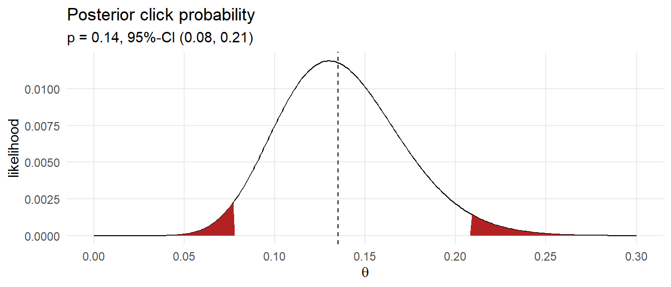
You can use a Bayesian model to estimate multiple parameters. Suppose you want to predict the water temperature in a lake on Jun 1 based on 5 years of prior water temperatures. You model the water temperature as a normal distribution, \(\mathrm{N}(\mu, \sigma)\) with a prior distribution \(\mu = \mathrm{N}(18, 5)\) and \(\sigma = \mathrm{unif}(0, 10)\) based on past experience.
Using the grid approximation approach, construct a grid of candidate \(\mu = [8.0, 8.5, \ldots, 30]\) and \(\sigma = [.1, .2, \ldots, 10]\) combinations - a 4,500 row data frame.
temp <- c(19, 23, 20, 17, 23)

# grid of proposed parameter values - parameter space
mdl_grid <- expand_grid(mu = seq(8, 30, by = 0.5),
                        sigma = seq(.1, 10, by = 0.1)) %>%
  mutate(mu_prior = map_dbl(mu, ~dnorm(., mean = 18, sd = 5)),
         sigma_prior = map_dbl(sigma, ~dunif(., 0, 10)),
         prior = mu_prior * sigma_prior, # combined prior,
         likelihood = map2_dbl(mu, sigma, ~dnorm(temp, .x, .y) %>% prod),
         posterior = likelihood * prior,
         posterior = posterior / sum(posterior))

mdl_grid %>%
  ggplot(aes(x = mu, y = sigma, fill = posterior)) +
  geom_tile() +
  scale_fill_gradient(low = "white", high = "steelblue", guide = "colorbar") +
  theme_minimal() +
  labs(title = "Joint probability of mu and sigma.",
       x = expression(mu), y = expression(sigma))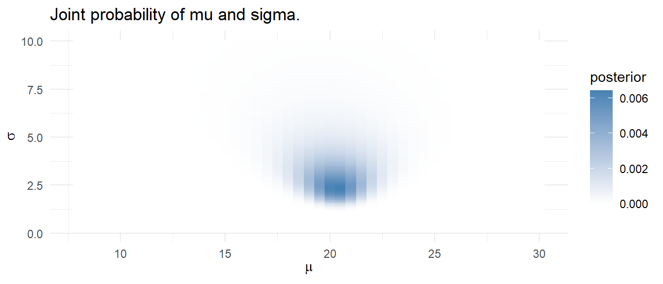
Calculate a credible interval by drawing 10,000 samples from the grid with sampling probability equal to the calculated posterior probabilities. Use the quantile() function to estimate the median and .025 and .975 quantile values.
sampling_idx <- sample(1:nrow(mdl_grid), size = 10000, replace = TRUE, prob = mdl_grid$posterior)
sampling_vals <- mdl_grid[sampling_idx, c("mu", "sigma")]
mu_ci <- quantile(sampling_vals$mu, c(.025, .5, .975))
sigma_ci <- quantile(sampling_vals$sigma, c(.025, .5, .975))
ci <- qnorm(c(.025, .5, .975), mean = mu_ci[2], sd = sigma_ci[2])

data.frame(temp = seq(0, 30, by = .1)) %>%
  mutate(prob = map_dbl(temp, ~dnorm(., mean = ci[2], sd = sigma_ci[2])),
         ci = if_else(temp >= ci[1] & temp <= ci[3], "Y", "N")) %>%
  ggplot(aes(x = temp, y = prob)) +
  geom_area(aes(y = if_else(ci == "N", prob, 0)),
            fill = "firebrick", show.legend = FALSE) +
  geom_line() +
  geom_vline(xintercept = ci[2], linetype = 2) +
  theme_minimal() +
  scale_x_continuous(breaks = seq(0, 30, 5)) +
  theme(panel.grid.minor = element_blank()) +
  labs(title = "Posterior temperature probability",
       subtitle = glue("mu = {ci[2] %>% scales::number(accuracy = .1)}, 95%-CI (",
       "{ci[1] %>% scales::number(accuracy = .1)}, ",
       "{ci[3] %>% scales::number(accuracy = .1)})"))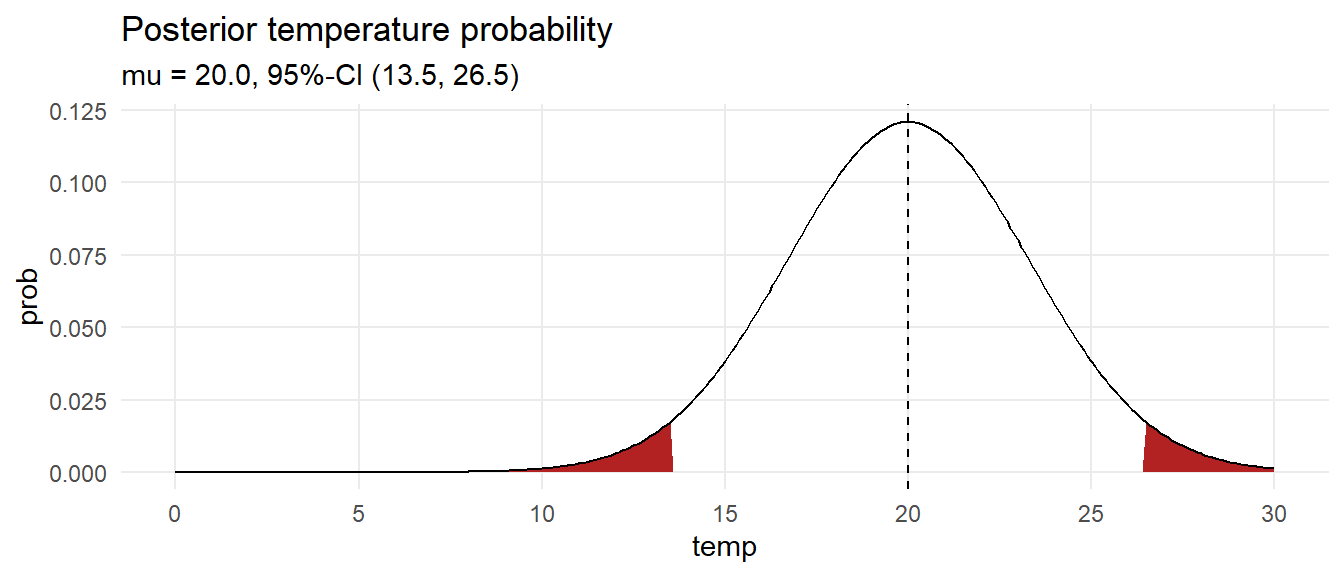
What is the probability the temperature is at least 18?
pred_temp <- rnorm(1000, mean = sampling_vals$mu, sampling_vals$sigma)
scales::percent(sum(pred_temp >= 18) / length(pred_temp))
## [1] "72%"Example borrowed from chris’ sandbox↩︎