12 Machine Learning
Go that way, really fast. If something gets in your way … turn.—Charles de Mar, “Better off Dead”
12.1 What is Machine Learning?
Machine learning (ML) is one of the most attractive skills you can have on a resume - it’s a complex, rapidly evolving field, taking advantage of continuing improvements in technology to accomplish increasingly difficult tasks. At the most abstract form, machine learning is just a way for computers to automatically make the same sort of models we’ve used in the past - by providing a large amount of data as an input, the machine can figure out which models give the best results, and “learn” how to improve its predictions without any human input. These models can be used for predictions - which customers will respond best to targeted ads; which areas need the most attention to prevent wildfires - or more complicated tasks, such as identifying the objects in images and the basic tasks associated with artifical intelligence.
We’re barely going to scratch the surface of machine learning - it’s a little deeper than most entry level jobs will require, and is beyond where most non-computational researchers are currently working. The goal isn’t to comprehensively cover all machine learning topics, as that’s a course in and of itself (usually taught a few years into a programming degree). Instead, we’ll be briefly covering the more basic and fundamental concepts - and how to implement them in R - in order to give you the tools and vocabulary you’ll need to learn more on your own.
12.2 Some Definitions
The first important piece of that vocabulary is knowing whether we’re asking a computer to perform supervised or unsupervised tasks. In both of these formats, we’re providing a large amount of data to an algorithm as an input to work with and learn from. In supervised learning, we’re then asking the computer to sort the data into a number of pre-defined classifications - for instance, is this email spam or not? What species is that tree?
With unsupervised learning, we’re asking the machine to find interesting patterns in the data by itself - this is what people mean when they refer to data mining.
There’s also a third type of learning, less applicable to the sort of work we’ve done in this course, known as reinforcement learning. This is what we use to teach robots to drive cars or play chess - certain outcomes are flagged as “good” or “bad”, so the machine starts avoiding the bad options and aiming for good ones.
We won’t be practicing any reinforcement or unsupervised techniques today. Instead, we’ll just do a brief overview of the most common supervised learning techniques.
12.3 Supervised Learning
Supervised learning tasks can be further broken into two factions:
- Classification problems, where the output is a category (spam/not spam, species of tree).
- Regression problems, where the output is a number (height, length).
You might recognize these as types of problems we’ve seen before - classification problems are natural fits for logistic models, while regression problems can be solved with linear modelling. In fact, these simpler models are the most basic forms of machine learning, and are sometimes better solutions to problems than these more modern techniques!
12.3.1 Classification
12.3.1.1 k-Nearest Neighbors
You might remember using logistic models in Unit 6 in order to predict a binary outcome - in that example, whether someone would win an Olympic medal. That model was relatively fast and effective, but had one pretty major downside - we could only predict whether someone won or not, rather than what sort of medal they had earned.
This is a pretty classic classification problem - we want to know what class each observation falls into, not just a binary outcome. We’ll be using the iris dataset to walk through the ML approach to this sort of problem, looking to predict what species a flower is by the measured variables. Remember that this dataset looks like the following:
head(iris)## Sepal.Length Sepal.Width Petal.Length Petal.Width Species
## 1 5.1 3.5 1.4 0.2 setosa
## 2 4.9 3.0 1.4 0.2 setosa
## 3 4.7 3.2 1.3 0.2 setosa
## 4 4.6 3.1 1.5 0.2 setosa
## 5 5.0 3.6 1.4 0.2 setosa
## 6 5.4 3.9 1.7 0.4 setosaWe’re going to be walking through the steps necessary to use the k-Nearest Neighbors algorithm to classify our dataset. This algorithm makes class predictions based on the known attributes of the data used to build the model - if setosa flowers have tiny petals, for instance, an unknown flower with tiny petals will probably be a setosa.
To do this, the algorithm finds the k nearest neighbors of each unknown data point - that is, the k known data points closest to the one we’re making predictions for, where k is a number that we get to define ourselves as best fits our datasets. To do this, the machine will first find the distance between datapoints by calculating the difference in each of their variables.
This is where some very cool packages come in - in this case, the package caret. Let’s install it now - warning, this could take a minute:
install.packages("caret")library(caret)## Loading required package: lattice## Loading required package: ggplot2The first thing we have to do is split our data into two sets - the training set, which will build the model, and the test set, which will evaluate its performance. To do so, we first have to randomly select which observations will go into each dataset.
Now, randomness is a complicated thing that’s incredibly hard for a computer to compute. But funnily enough, we really don’t want to purely randomly split our data up. If we did that, our work would be unreplicable, and our results would change every time we loaded R back up.
Instead, we want numbers that are random enough that we as humans can’t predict them - that way we can’t bias our results - but are replicable by a computer. These are called pseudorandom numbers, and we can control exactly what set we use by specifying set.seed() earlier in our code. So long as you’re working from the same seed, you should get the same sequence of random numbers as other researchers.
We then want to partition, or split, our data into training and test datasets. We can do so using createDataPartition() from caret, specifying what we want to split (the species in our dataset), what proportion of the data should make up each set (0.75 in the training and 0.25 in the test, in this case - you’ll frequently see between 60 and 80 percent of data being used for training), and how we want our output (in this example, a matrix, not a list):
set.seed(42)
index <- createDataPartition(iris$Species, p = 0.75, list = FALSE)
head(index)
## Resample1
## [1,] 1
## [2,] 3
## [3,] 4
## [4,] 5
## [5,] 6
## [6,] 7Now we have an index as an output, which is a matrix of numbers we’ll use to subdivide our data in the next step. Specifically, we’ll make a training dataset by selecting all the rows present in index, and a test dataset by selecting the rows which aren’t:
irisTrain <- iris[index, ]
irisTest <- iris[-index, ]
Feel free to inspect those datasets if you want confirmation that this worked the way it should have.
Now it’s time to train our model! Models in caret are built using the train() function, which works similarly to glm(). We’ll still specify our formula and data in the same format, and the type of model we want (though now we’ll use method = rather than family =). There are only two big differences with this format:
- Instead of specifying predictor variables in our formula, we’ll use
.to tell the algorithm to use all the data available to it - We’ll be specifying two preprocessing options - that we want to center and scale our data
That second one is a key step in kNN modeling. Remember that kNN calculates the distance between the variables of your training dataset and the point that it’s trying to predict. As such, variables with larger ranges can sometimes overpower a prediction - there’s a lot more distance to measure if your range is 1 to 1,000,000 than 1 to 10! As such, we’re going to rescale our data inside the training model, in order to treat all our variables equally. This all adds up to an equation that looks like this:
train(Species ~ ., data = irisTrain, method = "knn", preProcess = c("center", "scale"))## k-Nearest Neighbors
##
## 114 samples
## 4 predictor
## 3 classes: 'setosa', 'versicolor', 'virginica'
##
## Pre-processing: centered (4), scaled (4)
## Resampling: Bootstrapped (25 reps)
## Summary of sample sizes: 114, 114, 114, 114, 114, 114, ...
## Resampling results across tuning parameters:
##
## k Accuracy Kappa
## 5 0.9428585 0.9128917
## 7 0.9441087 0.9150565
## 9 0.9413363 0.9106879
##
## Accuracy was used to select the optimal model using the largest value.
## The final value used for the model was k = 7.That’s a pretty cool output, and one that’s easy to get excited about. What we just did was resample from our training set 25 times, fitting a different model each time. The best model from those 25 iterations is the k value specified at the bottom of the output.
You might notice that by re-running your code, you’ll sometimes get different results, but they all have about 90% accuracy. That’s because none of our models are dramatically better than any other - with larger datasets, you’ll often see a few models function significantly better than the other options. Here, all of ours are generally within a percentage point of each other.
We can’t report any of these results yet, however. We still have to test our model out on our test dataset!
To do this, we have to take three steps:
- Factor the species vector in the
irisTestdataset, so that our code works - Make predictions from our
knnModel, testing it against ouririsTestdataset - Make a confusion matrix, comparing the predicted results to our known values
Those first two steps are pretty easy:
knnModel <- train(Species ~ ., data = irisTrain, method = "knn", preProcess = c("center", "scale"))
irisTest$Species <- factor(irisTest$Species)
knnPredict <- predict(knnModel, newdata = irisTest)
And now we do the more, well, confusing part of that. Let’s use confusionMatrix() with our predicted and actual variables as arguments, then we’ll walk through what exactly we did:
confusionMatrix(knnPredict, irisTest$Species)## Confusion Matrix and Statistics
##
## Reference
## Prediction setosa versicolor virginica
## setosa 12 0 0
## versicolor 0 11 3
## virginica 0 1 9
##
## Overall Statistics
##
## Accuracy : 0.8889
## 95% CI : (0.7394, 0.9689)
## No Information Rate : 0.3333
## P-Value [Acc > NIR] : 6.677e-12
##
## Kappa : 0.8333
## Mcnemar's Test P-Value : NA
##
## Statistics by Class:
##
## Class: setosa Class: versicolor Class: virginica
## Sensitivity 1.0000 0.9167 0.7500
## Specificity 1.0000 0.8750 0.9583
## Pos Pred Value 1.0000 0.7857 0.9000
## Neg Pred Value 1.0000 0.9545 0.8846
## Prevalence 0.3333 0.3333 0.3333
## Detection Rate 0.3333 0.3056 0.2500
## Detection Prevalence 0.3333 0.3889 0.2778
## Balanced Accuracy 1.0000 0.8958 0.8542What we’re looking at now are our actual results - this is what we’d report for our model. Our model is significantly better than the null model (that p value [Acc > NIR]), with about an 88.9% accuracy rate. We can also see exactly where our model gets confused - one versicolor flower was misclassed as virginica, while three virginica flowers were mis-classed as versicolor.
12.3.2 Support Vector Machines
kNN is only one of the several popular classification algorithms available in R. One of the newest - and most popular - methods is the support vector machine, or SVM.
Exactly what an SVM does is a little tricky to explain - so we’ll simplify things slightly, in order to make it a bit easier. Let’s say you have an assortment of data points:
## ── Attaching packages ──────────────────────────────────────────────────────────────────────────────────────── tidyverse 1.2.1 ──## ✔ tibble 1.4.2 ✔ purrr 0.2.5
## ✔ tidyr 0.8.2 ✔ dplyr 0.7.8
## ✔ readr 1.1.1 ✔ stringr 1.3.1
## ✔ tibble 1.4.2 ✔ forcats 0.3.0## ── Conflicts ─────────────────────────────────────────────────────────────────────────────────────────── tidyverse_conflicts() ──
## ✖ dplyr::filter() masks stats::filter()
## ✖ dplyr::lag() masks stats::lag()
## ✖ purrr::lift() masks caret::lift()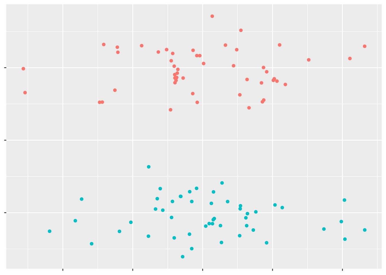
We can see a pretty obvious line to separate the two groups of points:
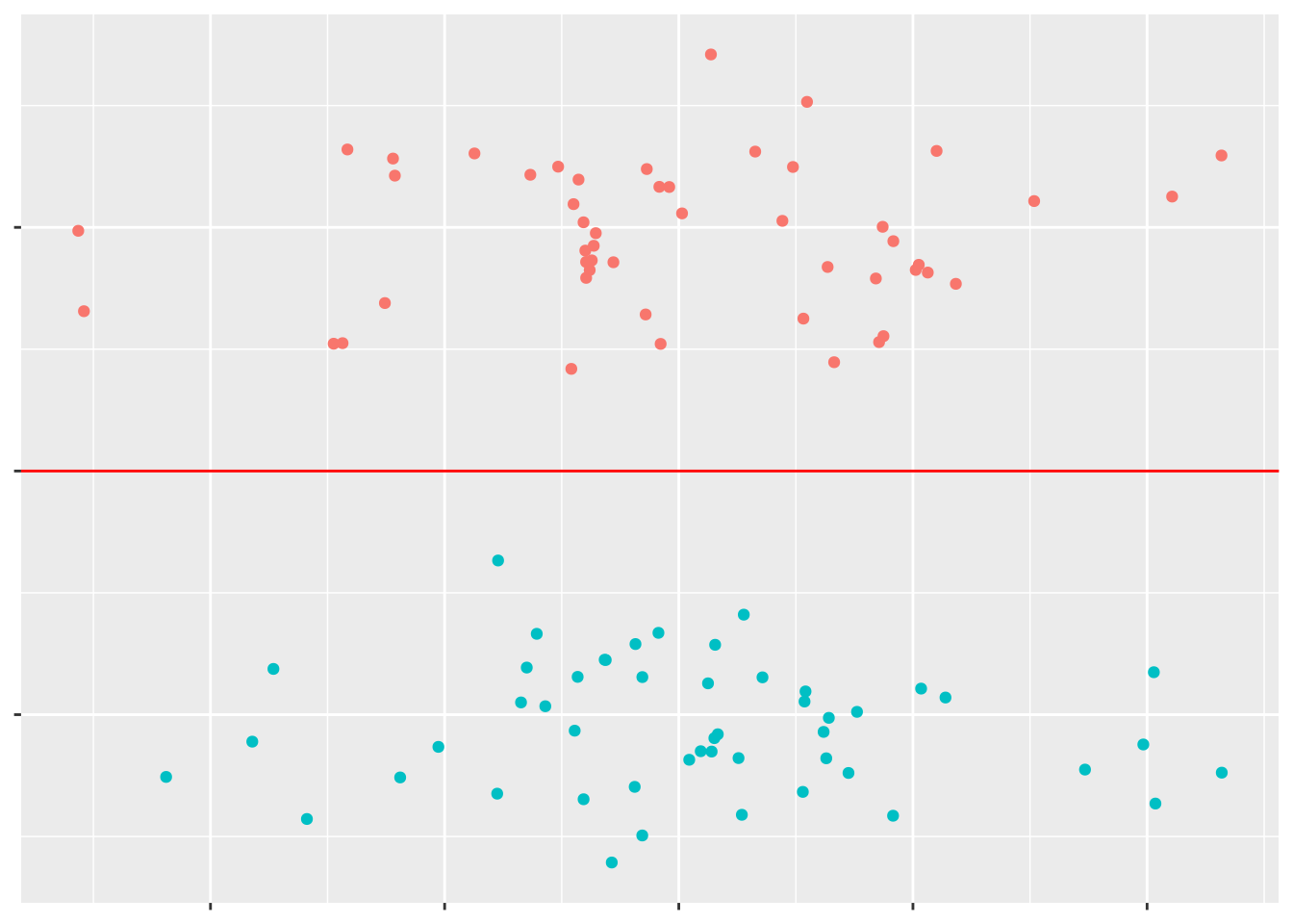
But if these points are a little more complicated, it can be harder to find the best line of separation.
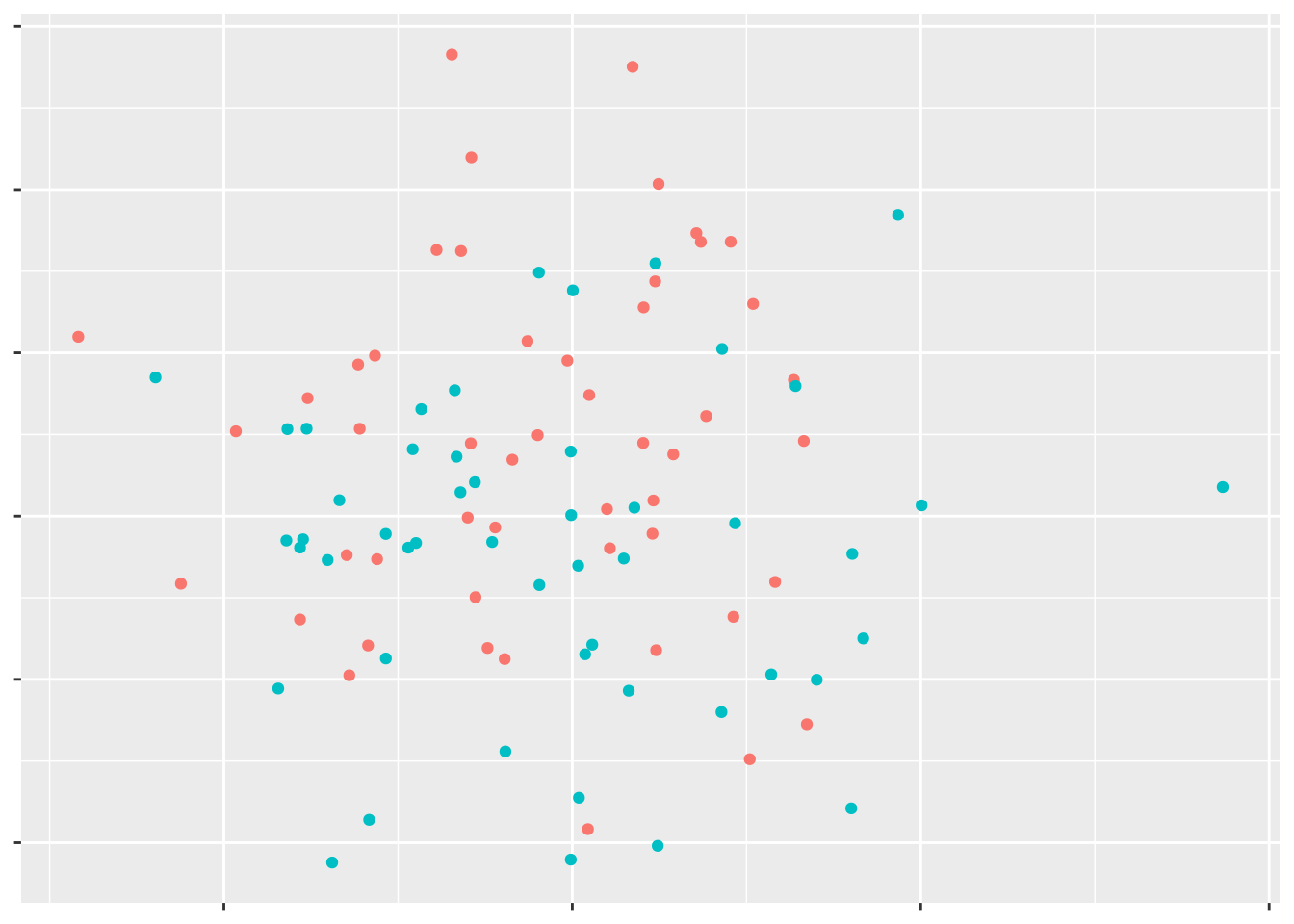
However, if we had a third variable for these data points, we might be able to find some line separating the data points:
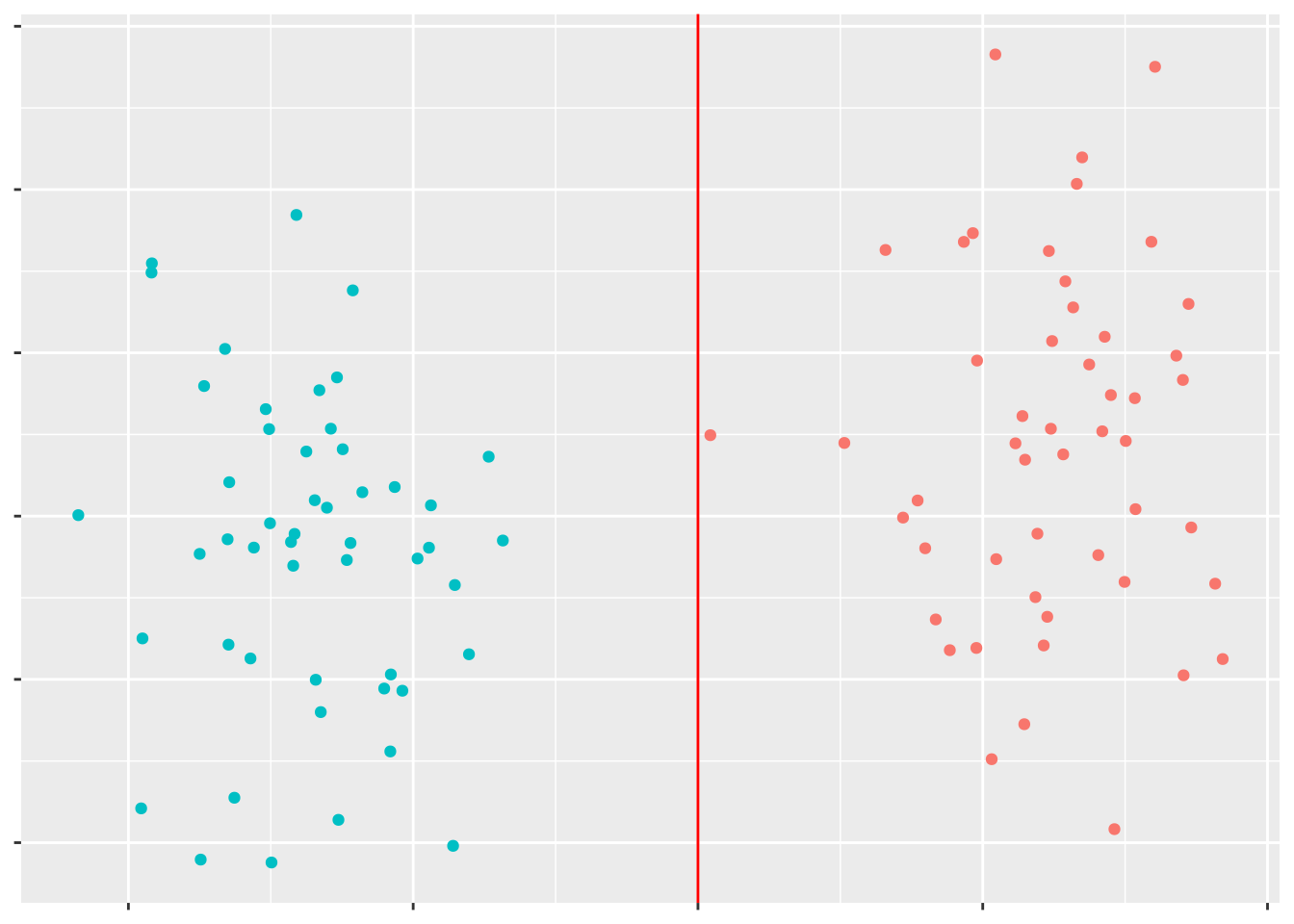
This is what SVMs do: find the best line (in hyperspace - basically, using as many dimensions as you have variables) to separate your data. The best implementation of SVMs in R comes from the e1071 package - let’s install that now:
install.packages("e1071")library(e1071)We then can train a SVM using the smv() command, in a similar fashion to the train() command from caret:
SVMFit <- svm(Species ~ ., data = iris)And then, just like before, we can assess our model using a confusion matrix:
SVMPredict <- predict(SVMFit, newdata = irisTest)
confusionMatrix(SVMPredict, irisTest$Species)
## Confusion Matrix and Statistics
##
## Reference
## Prediction setosa versicolor virginica
## setosa 12 0 0
## versicolor 0 11 2
## virginica 0 1 10
##
## Overall Statistics
##
## Accuracy : 0.9167
## 95% CI : (0.7753, 0.9825)
## No Information Rate : 0.3333
## P-Value [Acc > NIR] : 3.978e-13
##
## Kappa : 0.875
## Mcnemar's Test P-Value : NA
##
## Statistics by Class:
##
## Class: setosa Class: versicolor Class: virginica
## Sensitivity 1.0000 0.9167 0.8333
## Specificity 1.0000 0.9167 0.9583
## Pos Pred Value 1.0000 0.8462 0.9091
## Neg Pred Value 1.0000 0.9565 0.9200
## Prevalence 0.3333 0.3333 0.3333
## Detection Rate 0.3333 0.3056 0.2778
## Detection Prevalence 0.3333 0.3611 0.3056
## Balanced Accuracy 1.0000 0.9167 0.8958Almost 92% accuracy! That’s pretty awesome!
If you want a techier explanation of SVMs, check out this blog post by Savan Patel.
12.3.2.1 Decision Trees
Another of the most commonly used methods (kinda - we’ll get to that in a minute) is known as the decision tree. Basically, this method creates a flowchart with each of your variables - at each split in the chart (known as a “node”), the algorithm uses a selection of variables to try and classify your data. This technique makes use of the bootstrapping we discussed in the past unit - by increasing our sample size, we’re able to increase the predictive power of each tree.
We’re going to use the rpart package to make our decision trees for this unit. First, we have to install the package, then load it using library():
install.packages("rpart")library(rpart)And now we fit the tree much like we did for our kNN model. In fact, I’m going to use almost the exact same code as we did above, except for a few important differences. One of the biggest is including type = "class" in the predict() call - otherwise, we’ll get a table of the probability each flower is a given species, rather than a prediction.
TreeFit <- rpart(Species ~ ., data = irisTest)
TreeFit
## n= 36
##
## node), split, n, loss, yval, (yprob)
## * denotes terminal node
##
## 1) root 36 24 setosa (0.3333333 0.3333333 0.3333333)
## 2) Petal.Length< 2.5 12 0 setosa (1.0000000 0.0000000 0.0000000) *
## 3) Petal.Length>=2.5 24 12 versicolor (0.0000000 0.5000000 0.5000000)
## 6) Petal.Width< 1.65 14 2 versicolor (0.0000000 0.8571429 0.1428571) *
## 7) Petal.Width>=1.65 10 0 virginica (0.0000000 0.0000000 1.0000000) *TreePredict <- predict(TreeFit, newdata = irisTest, type = "class")
confusionMatrix(TreePredict, irisTest$Species)## Confusion Matrix and Statistics
##
## Reference
## Prediction setosa versicolor virginica
## setosa 12 0 0
## versicolor 0 12 2
## virginica 0 0 10
##
## Overall Statistics
##
## Accuracy : 0.9444
## 95% CI : (0.8134, 0.9932)
## No Information Rate : 0.3333
## P-Value [Acc > NIR] : 1.728e-14
##
## Kappa : 0.9167
## Mcnemar's Test P-Value : NA
##
## Statistics by Class:
##
## Class: setosa Class: versicolor Class: virginica
## Sensitivity 1.0000 1.0000 0.8333
## Specificity 1.0000 0.9167 1.0000
## Pos Pred Value 1.0000 0.8571 1.0000
## Neg Pred Value 1.0000 1.0000 0.9231
## Prevalence 0.3333 0.3333 0.3333
## Detection Rate 0.3333 0.3333 0.2778
## Detection Prevalence 0.3333 0.3889 0.2778
## Balanced Accuracy 1.0000 0.9583 0.916794.4% accuracy! It’s important to note exactly what’s changed since last time - we’ve classified two flowers better, which - on this small dataset - means we were incredibly more predictive.
However, decision trees on their own aren’t particularly great classifiers. For one thing, they tend to overfit the data, making your model less applicable to other datasets. They also generally require a decent amount of tuning to be optimally accurate. Luckily, there’s a better way to classify your data than using a single tree:
12.3.2.2 Random Forests
Random forests!
These forests are collections of trees (get it?), all of which may overfit the data in some weird way and have oddly bad fits in others. The idea is to collect as many trees as we can in one model and find out what the majority of models want to classify the datapoint as - by aggregating large numbers of trees, we can avoid the pitfalls that individual trees tend to lead us towards. These random forests also randomize the variables used in each tree, increasing the applicability of the model to different datasets.
There’s a ton of random forest implementations in R, because these are some of the most current and useful ML applications we’ve developed so far. I’m going to, for the sake of simplicity, stick with one of the better-known applications. We’ll keep using our functions from caret(), but first, we have to install the ranger application:
install.packages("ranger")We can now use the exact same code as our kNN model to fit a random forest model to our data and test its accuracy. The only difference is that this time, we’re using method = "ranger":
ForestFit <- train(Species ~ ., data = irisTrain, method = "ranger")
ForestFit
## Random Forest
##
## 114 samples
## 4 predictor
## 3 classes: 'setosa', 'versicolor', 'virginica'
##
## No pre-processing
## Resampling: Bootstrapped (25 reps)
## Summary of sample sizes: 114, 114, 114, 114, 114, 114, ...
## Resampling results across tuning parameters:
##
## mtry splitrule Accuracy Kappa
## 2 gini 0.9600118 0.9391308
## 2 extratrees 0.9664561 0.9488236
## 3 gini 0.9610118 0.9406517
## 3 extratrees 0.9701867 0.9544365
## 4 gini 0.9591513 0.9379683
## 4 extratrees 0.9675020 0.9503870
##
## Tuning parameter 'min.node.size' was held constant at a value of 1
## Accuracy was used to select the optimal model using the largest value.
## The final values used for the model were mtry = 3, splitrule =
## extratrees and min.node.size = 1.ForestPredict <- predict(ForestFit, irisTest)
confusionMatrix(ForestPredict, irisTest$Species)## Confusion Matrix and Statistics
##
## Reference
## Prediction setosa versicolor virginica
## setosa 12 0 0
## versicolor 0 12 3
## virginica 0 0 9
##
## Overall Statistics
##
## Accuracy : 0.9167
## 95% CI : (0.7753, 0.9825)
## No Information Rate : 0.3333
## P-Value [Acc > NIR] : 3.978e-13
##
## Kappa : 0.875
## Mcnemar's Test P-Value : NA
##
## Statistics by Class:
##
## Class: setosa Class: versicolor Class: virginica
## Sensitivity 1.0000 1.0000 0.7500
## Specificity 1.0000 0.8750 1.0000
## Pos Pred Value 1.0000 0.8000 1.0000
## Neg Pred Value 1.0000 1.0000 0.8889
## Prevalence 0.3333 0.3333 0.3333
## Detection Rate 0.3333 0.3333 0.2500
## Detection Prevalence 0.3333 0.4167 0.2500
## Balanced Accuracy 1.0000 0.9375 0.8750Our accuracy is lower! How could that be?
As it happens, that’s almost a good thing in this situation. While the decision tree we made earlier was extremely accurate on the small dataset we tested it on, in most situations these trees will falter when presented with new data. The lower accuracy represented here means that the model may not be as good a fit for our data, but it’s likely more generalizable as a result.
If we want a little bit more information about our forest, we can call ForestFit$finalModel for a few extra details:
ForestFit$finalModel## Ranger result
##
## Call:
## ranger::ranger(dependent.variable.name = ".outcome", data = x, mtry = param$mtry, min.node.size = param$min.node.size, splitrule = as.character(param$splitrule), write.forest = TRUE, probability = classProbs, ...)
##
## Type: Classification
## Number of trees: 500
## Sample size: 114
## Number of independent variables: 4
## Mtry: 3
## Target node size: 1
## Variable importance mode: none
## Splitrule: extratrees
## OOB prediction error: 2.63 %This tells us that we’ve built 500 decision trees for our training sample of 114 observations, using all 4 predictors in at least some of the trees, with 2 variables used in each individual tree.
12.3.3 Regression Models
For this next section, we’ll be working with a dataset contained in the MASS package:
install.packages("MASS")library(MASS)##
## Attaching package: 'MASS'## The following object is masked from 'package:dplyr':
##
## selectThis package contains a bunch of datasets for a 2002 textbook. We’ll be using the Boston dataset to predict median home prices based on neighborhood demographics and traits. Let’s look at our dataset:
head(Boston)## crim zn indus chas nox rm age dis rad tax ptratio black
## 1 0.00632 18 2.31 0 0.538 6.575 65.2 4.0900 1 296 15.3 396.90
## 2 0.02731 0 7.07 0 0.469 6.421 78.9 4.9671 2 242 17.8 396.90
## 3 0.02729 0 7.07 0 0.469 7.185 61.1 4.9671 2 242 17.8 392.83
## 4 0.03237 0 2.18 0 0.458 6.998 45.8 6.0622 3 222 18.7 394.63
## 5 0.06905 0 2.18 0 0.458 7.147 54.2 6.0622 3 222 18.7 396.90
## 6 0.02985 0 2.18 0 0.458 6.430 58.7 6.0622 3 222 18.7 394.12
## lstat medv
## 1 4.98 24.0
## 2 9.14 21.6
## 3 4.03 34.7
## 4 2.94 33.4
## 5 5.33 36.2
## 6 5.21 28.7That last column, medv, is the one that we’re interested in predicting. If you want to know what the other variables mean, try ?Boston.
BostonIndex <- createDataPartition(Boston$medv, p = 0.75, list = FALSE)

BostonTrain <- Boston[BostonIndex, ]
BostonTest <- Boston[-BostonIndex, ]
Now, historically, we’d predict medv with a regression model, such as a linear model.
BostonLinear <- lm(medv ~ ., data = Boston)We can then find the R2 value for that model (or, if you want all the model statistics, cut all the text after the right parenthesis):
summary(BostonLinear)$r.sq## [1] 0.7406427And that’s pretty successful! Not perfect, but successful enough.
If we build a random forest, meanwhile, following the same steps as above:
BostonForest <- train(medv ~ ., data = BostonTrain, method = "ranger")
BostonForest
## Random Forest
##
## 381 samples
## 13 predictor
##
## No pre-processing
## Resampling: Bootstrapped (25 reps)
## Summary of sample sizes: 381, 381, 381, 381, 381, 381, ...
## Resampling results across tuning parameters:
##
## mtry splitrule RMSE Rsquared MAE
## 2 variance 4.198524 0.8074691 2.682807
## 2 extratrees 4.680094 0.7682666 2.988957
## 7 variance 3.810779 0.8303916 2.448718
## 7 extratrees 3.953657 0.8221902 2.473085
## 13 variance 3.960433 0.8144638 2.560585
## 13 extratrees 3.923580 0.8211972 2.458137
##
## Tuning parameter 'min.node.size' was held constant at a value of 5
## RMSE was used to select the optimal model using the smallest value.
## The final values used for the model were mtry = 7, splitrule =
## variance and min.node.size = 5.We can see that our best model has an R2 around 85%! Even better!
Now, there’s a lot of discussion about whether or not you need to have separate training and testing datasets with random forest datasets. A lot of this conversation concerns data with tens of thousands of observations, if not more - in those cases, the random forest will automatically use about 2/3 of the data to build each model, and will report R2 values that theoretically reflect how the model does with new data.
With our tiny data, however, we can see that each model is built with the entirety of the dataset. As such, it’s still worth splitting our data, in order to get more accurate representations of how our model does with new data. To do so, I’m going to build a new function to calculate R2, following the equation: \[R^2 = 1 - \frac{\sum (y - \hat{y})^2}{\sum (y - \bar{y})^2} \]
Which, in our code, looks like this:
rsqcalc <- function(y, predicted){
  1 - sum((y - predicted)^2)/sum((y - mean(y))^2)
}
Then generate predictions for our training dataset, and use this new function to find the R2:
BostonTest$Predicted <- predict(BostonForest, BostonTest)
rsqcalc(BostonTest$medv, BostonTest$Predicted)
## [1] 0.914374Even higher!
We aren’t going to get further into supervised learning methods, as other methods - such as neural networks - require a little more conceptual backing than I’m willing to dive into in this space. If you want to learn more, the textbook Introduction to Statistical Learning is a good place to start, with a free PDF online.
Note, by the way, that we are barely scratching the surface of what caret can do - there’s a full book on this package at this link, though fair warning, it’s a little intimidating.
12.4 Unsupervised Learning
By contrast to supervised learning, unsupervised learning does not make predictions on new groups. Instead, the focus of unsupervised techniques is to discover patterns in the data - to see if there are groups or patterns to be identified in the variables you have collected. It can often be used as a part of exploratory analyses and inspire further questions.
If that all sounds rather squishy to you, it is - which is one of the hardest parts about unsupervised techniques. As there is no obvious metric to objectively evaluate these models - after all, we aren’t making predictions, so there’s no use for test datasets in evaluating our outputs - and no obvious true answer we can gut-check against.
As such, unsupervised learning can be incredibly difficult, and requires a strong background in other statistical analyses - putting it somewhat beyond the scope of this reader. If you’re interested in learning more, chapters 6 and 10 of Introduction to Statistical Learning provide a great introduction using R.