Chapter 2 Working with vectores, matrices, and arrays

2.1 Data objects in R

2.1.1 Atomic vs. recursive data objects

The analysis of data in R involves creating, naming, manipulating, and operating on data objects using functions. Data in R are organized as objects and have been assigned names. We have already been introduced to several R data objects. We now make further distinctions. Every data object has a mode and length. The mode of an object describes the type of data it contains and is available by using the mode function. An object can be of mode character, numeric, logical, list, or function.

fname <- c('Juan', 'Miguel'); mode(fname)

## [1] "character"

age <- c(34, 20); mode(age)

## [1] "numeric"

lt25 <- age<25; lt25 

## [1] FALSE  TRUE

mode(lt25)

## [1] "logical"

mylist <- list(fname, age); mode(mylist)

## [1] "list"

mydat <- data.frame(fname, age); mode(mydat)

## [1] "list"

myfun <- function(x) {x^2}
myfun(5)

## [1] 25

mode(myfun)

## [1] "function"

Data objects are further categorized into atomic or recursive objects. An atomic data object can only contain elements from one, and only one, of the following modes: character, numeric, or logical. Vectors, matrices, and arrays are atomic data objects. A recursive data object can contain data objects of any mode. Lists, data frames, and functions are recursive data objects. We start by reviewing atomic data objects. A vector is a collection of like elements without dimensions.⁶ The vector elements are all of the same mode (either character, numeric, or logical). When R returns a vector the [n] indicates the position of the element displayed to its immediate right.

y <- c('Pedro', 'Paulo', 'Maria'); y # character

## [1] "Pedro" "Paulo" "Maria"

x <- c(1, 2, 3, 4, 5); x             # numeric

## [1] 1 2 3 4 5

x < 3                                # logical

## [1]  TRUE  TRUE FALSE FALSE FALSE

A matrix is a collection of like elements organized into a 2-dimensional (tabular) data object. We can think of a matrix as a vector with a 2-dimensional structure. When R returns a matrix the [n,] indicates the nth row and [,m] indicates the mth column.

x <- c('a', 'b', 'c', 'd')
y <- matrix(x, 2, 2); y

##      [,1] [,2]
## [1,] "a"  "c" 
## [2,] "b"  "d"

An array is a collection of like elements organized into a n-dimensional data object. We can think of an array as a vector with an n-dimensional structure. When R returns an array the [n,,] indicates the nth row and [,m,] indicates the mth column, and so on.

x <- 1:8
y <- array(x, dim=c(2, 2, 2)); y

## , , 1
## 
##      [,1] [,2]
## [1,]    1    3
## [2,]    2    4
## 
## , , 2
## 
##      [,1] [,2]
## [1,]    5    7
## [2,]    6    8

If we try to include elements of different modes in an atomic data object, R will coerce the data object into a single mode based on the following hierarchy: character \(>\) numeric \(>\) logical. In other words, if an atomic data object contains any character element, all the elements are coerced to character.

c('hello', 4.56, FALSE)

## [1] "hello" "4.56"  "FALSE"

c(4.56, FALSE)

## [1] 4.56 0.00

A recursive data object can contain one or more data objects where each object can be of any mode. Lists, data frames, and functions are recursive data objects. Lists and data frames are of mode list, and functions are of mode function (Table 2.1).

A list is a collection of data objects without any restrictions:

x <- c(1, 2, 3)                   # numeric vector
y <- c('Male', 'Female', 'Male')  # character vector
z <- matrix(1:4, 2, 2)            # numemric matrix
mylist <- list(x, y, z); mylist   # list

## [[1]]
## [1] 1 2 3
## 
## [[2]]
## [1] "Male"   "Female" "Male"  
## 
## [[3]]
##      [,1] [,2]
## [1,]    1    3
## [2,]    2    4

A data frame is a list with a 2-dimensional (tabular) structure. Epidemiologists are very experienced working with data frames where each row usually represents data collected on individual subjects (also called records or observations) and columns represent fields for each type of data collected (also called variables).

subjno <- c(1, 2, 3, 4)
age <- c(34, 56, 45, 23)
sex <- c('Male', 'Male', 'Female', 'Male')
case <- c('Yes', 'No', 'No', 'Yes')
mydat <- data.frame(subjno, age, sex, case); mydat

##   subjno age    sex case
## 1      1  34   Male  Yes
## 2      2  56   Male   No
## 3      3  45 Female   No
## 4      4  23   Male  Yes

mode(mydat)

## [1] "list"

2.1.2 Assessing the structure of data objects

Table 2.1: Summary of six types of data objects in R

Data object	Possible mode	Default class
Atomic
vector	character, numeric, logical	NULL
matrix	character, numeric, logical	NULL
array	character, numeric, logical	NULL
Recursive
list	list	NULL
data frame	list	data frame
function	function	NULL

Summarized in Table 2.1 are the key attributes of atomic and recursive data objects. Data objects can also have class attributes. Class attributes are just a way of letting R know that an object is ‘special,’ allowing R to use specific methods designed for that class of objects (e.g., print, plot, and summary methods). The class function displays the class if it exists. For our purposes, we do not need to know any more about classes.

Frequently, we need to assess the structure of data objects. We already know that all data objects have a mode and length attribute. For example, let’s explore the infert data set that comes with R. The infert data comes from a matched case-control study evaluating the occurrence of female infertility after spontaneous and induced abortion.

data(infert) # loads data 
mode(infert)

## [1] "list"

length(infert)

## [1] 8

At this point we know that the data object named ‘infert’ is a list of length 8. To get more detailed information about the structure of infert use the str function (str comes from ’str’ucture).

str(infert)

## 'data.frame':    248 obs. of  8 variables:
##  $ education     : Factor w/ 3 levels "0-5yrs","6-11yrs",..: 1 1 1 1 2 2 2 2 2 2 ...
##  $ age           : num  26 42 39 34 35 36 23 32 21 28 ...
##  $ parity        : num  6 1 6 4 3 4 1 2 1 2 ...
##  $ induced       : num  1 1 2 2 1 2 0 0 0 0 ...
##  $ case          : num  1 1 1 1 1 1 1 1 1 1 ...
##  $ spontaneous   : num  2 0 0 0 1 1 0 0 1 0 ...
##  $ stratum       : int  1 2 3 4 5 6 7 8 9 10 ...
##  $ pooled.stratum: num  3 1 4 2 32 36 6 22 5 19 ...

Great! This is better. We now know that infert is a data frame with 248 observations and 8 variables. The variable names and data types are displayed along with their first few values. In this case, we now have sufficient information to start manipulating and analyzing the infert data set.

Additionally, we can extract more detailed structural information that becomes useful when we want to extract data from an object for further manipulation or analysis (Table 2.2). We will see extensive use of this when we start programming in R.

To get practice calling data from the console, enter data() to display the available data sets in R. Then enter data(data_set) to load a dataset. Study the examples in Table 2.2 and spend a few minutes exploring the structure of the data sets we have loaded. To display detailed information about a specific data set use ?data_set at the command prompt (e.g., ?infert).

Table 2.2: Useful functions for assessing R data objects

Function	Description	Try these examples
Returns summary objects
str	Displays summary of data object structure	str(infert)
attributes	Returns list with data object attributes	attributes(infert)
Returns specific information
mode	Returns mode of object	mode(infert)
class	Returns class of object, if it exists	class(infert)
length	Returns length of object	length(infert)
dim	Returns vector with object dimensions, if applicable	dim(infert)
nrow	Returns number of rows, if applicable	nrow(infert)
ncol	Returns number of columns, if applicable	ncol(infert)
dimnames	Returns list containing vectors of names for each dimension, if applicable	dimnames(infert)
rownames	Returns vector of row names of a matrix-like object	rownames(infert)
colnames	Returns vector of column names of a matrix-like object	colnames(infert)
names	Returns vector of names for the list (for a data frame returns field names)	names(infert)
row.names	Returns vector of row names for a data frame	row.names(infert)

2.2 A vector is a collection of like elements

2.2.1 Understanding vectors

A vector is a collection of like elements (i.e., the elements all have the same mode). There are many ways to create vectors (see Table 2.5). The most common way of creating a vector is using the c function:

chol <- c(136, 219, 176, 214, 164); chol     # numeric

## [1] 136 219 176 214 164

fn <- c('Mateo', 'Mark', 'Luke', 'Juan'); fn # character

## [1] "Mateo" "Mark"  "Luke"  "Juan"

z <- c(T, T, F, T, F); z                     # logical

## [1]  TRUE  TRUE FALSE  TRUE FALSE

A single element is also a vector; that is, a vector of length = 1. Try, for example, is.vector('Zoe'). In mathematics, a single number is called a scalar; in R, it is a numeric vector of length = 1. When we execute a math operation between a scalar and a vector, in the background, the scalar expands to the same length as the vector in order to execute a vectorized operation. For example, these two calculation are equivalent:

x1 <- 5; y1 <- c(10, 20, 30)
x2 <- c(5, 5, 5); y2 <- c(10, 20, 30)
x1 * y1

## [1]  50 100 150

x2 * y2

## [1]  50 100 150

A note of caution: when vector lengths differ, the shorter vector will recyle its elements to enable a vectorized operation. For example,

x <- c(3, 5); y = c(10, 20, 30, 40)
z <- x * y     # multipy vectors with different lengths
cbind(x, y, z) # display results

##      x  y   z
## [1,] 3 10  30
## [2,] 5 20 100
## [3,] 3 30  90
## [4,] 5 40 200

In effect, x expanded from c(3, 5) to c(3, 5, 3, 5) in order to execute a vectorized operation. This expansion of x is not apparent from the math operation; that is, no warning was produced. Therefore, be aware: math operations with vectors of different lengths may not produce a warning.

2.2.1.1 Boolean operations on vectors

In R, we use relational and logical operators (Table 2.3) and (Table 2.4) to conduct Boolean queries. Boolean operations is a methodological workhorse of data analysis. For example, suppose we have a vector of female movie stars and a corresponding vector of their ages (as of January 16, 2004), and we want to select a subset of actors based on age criteria. Let’s select the actors who are in their 30s. This is done using logical vectors that are created by using relational operators (<, >, <=, >=, ==, !=). Study the following example:

movie.stars <- c('Rebecca De Mornay', 'Elisabeth Shue', 'Amanda Peet',
  'Jennifer Lopez', 'Winona Ryder', 'Catherine Zeta Jones', 'Reese Witherspoon')
ms.ages <- c(42, 40, 32, 33, 32, 34, 27)
ms.ages >= 30 # logical vector for stars with ages >=30 

## [1]  TRUE  TRUE  TRUE  TRUE  TRUE  TRUE FALSE

ms.ages < 40 # logical vector for stars with ages <40 

## [1] FALSE FALSE  TRUE  TRUE  TRUE  TRUE  TRUE

(ms.ages >= 30) & (ms.ages < 40) # intersection of vectors

## [1] FALSE FALSE  TRUE  TRUE  TRUE  TRUE FALSE

thirtysomething <- (ms.ages >= 30) & (ms.ages < 40)
movie.stars[thirtysomething] # indexing using logical

## [1] "Amanda Peet"          "Jennifer Lopez"       "Winona Ryder"        
## [4] "Catherine Zeta Jones"

Table 2.3: Using relational operators with vectors

Operator	Description	Try these examples
<	Less than	pos <- c('p1', 'p2', 'p3', 'p4')
		x <- c(1, 2, 3, 4)
		y <- c(5, 4, 3, 2)
		x < y
		pos[x < y]
>	Greater than	x > y
		pos[x > y]
<=	Less than or equal to	x <= y
		pos[x <= y]
>=	Greater than or equal to	x >= y
		pos[x >= y]
==	Equal to	x == y
		pos[x == y]
!=	Not equal to	x != y
		pos[x != y]

Table 2.4: Using logical operators with vectors

Operator	Description	Try these examples
!	Element-wise NOT	x <- c(1, 2, 3, 4)
		x > 2
		!(x > 2)
		pos[!(x > 2)]
&	Element-wise AND	(x > 1) & (x < 5)
		pos[(x > 1) & (x < 5)]
\(\mid\)	Element-wise OR	(x <= 1) \(\mid\) (x > 4)
		pos[(x <= 1) \(\mid\) (x > 4)]
xor	Exclusive OR: only TRUE if one or other element is true, not both	xx <- x <= 1
		yy <- x > 4
		xor(xx, yy)

To summarize: - Logical vectors are created using Boolean comparisons, - Boolean comparisons are constructed using relational and logical operators - Logical vectors are commonly used for indexing (subsetting) data objects

Before moving on, we need to be sure we understand the previous examples, then study the examples in the Table 2.3 and Table 2.4. For practice, study the examples and spend a few minutes creating simple numeric vectors, then (1) generate logical vectors using relational operators, (2) use these logical vectors to index the original numerical vector or another vector, (3) generate logical vectors using the combination of relational and logical operators, and (4) use these logical vectors to index the original numerical vector or another vector.

Notice that the element-wise exclusive or operator (xor) returns TRUE if either comparison element is TRUE, but not if both are TRUE. In contrast, the | returns TRUE if either or both comparison elements are TRUE.

2.2.2 Creating vectors

Table 2.5: Common ways of creating vectors de novo

Function	Description	Try these examples
c	Concatenate a collection	x <- c(1, 2, 3, 4, 5)
		y <- c(6, 7, 8, 9, 10)
		z <- c(x, y)
scan	Scan a collection	xx <- scan()
		1 2 3 4 5 # Press Enter twice
		yy <- scan(what = '')
		'Javier' 'Miguel' 'Martin' # Press Enter twice
		xx; yy # Display vectors
:	Generate integer sequence	1:10
		10:(-4)
seq	Generate sequence of numbers	seq(1, 5, by = 0.5)
		seq(1, 5, length = 3)
		zz <- c('a', 'b', 'c')
		seq(along = zz)
rep	Replicate argument	rep('Juan Nieve', 3)
		rep(1:3, 4)
		rep(1:3, 3:1)
paste	Paste character string elements	paste(c('A','B','C'),1:3,sep='')

%% TODO add sample, rnorm, which, numeric

Vectors are created directly, or indirectly as the result of manipulating an R object. The c function for concatenating a collection has been covered previously. Another, possibly more convenient, method for collecting elements into a vector is with the scan function.

> x <- scan()
1:  45 67 23 89
5: 
Read 4 items
> x
[1] 45 67 23 89             

This method is convenient because we do not need to type c, parentheses, and commas to create the vector. The vector is created after executing a newline twice.

To generate a sequence of consecutive integers use the : function.

-9:8

##  [1] -9 -8 -7 -6 -5 -4 -3 -2 -1  0  1  2  3  4  5  6  7  8

However, the seq function provides more flexibility in generating sequences. Here are some examples:

seq(1, 5, by = 0.5)    # specify interval

## [1] 1.0 1.5 2.0 2.5 3.0 3.5 4.0 4.5 5.0

seq(1, 5, length = 8)  # specify length

## [1] 1.000000 1.571429 2.142857 2.714286 3.285714 3.857143 4.428571 5.000000

x <- 1:8
seq(1, 5, along = x)   # by length of other object

## [1] 1.000000 1.571429 2.142857 2.714286 3.285714 3.857143 4.428571 5.000000

These types of sequences are convenient for plotting mathematical equations.⁷ For example, suppose we wanted to plot the standard normal curve using the normal equation. For a standard normal curve \(\mu = 0\) (mean) and \(\sigma = 1\) (standard deviation)

\[\begin{equation} f(x) = \frac{1}{\sqrt{2 \pi \sigma^2}} \exp \left\{\frac{-(x - \mu)^2}{2 \sigma^2} \right\} \end{equation}\]

Here is the R code to plot this equation:

mu <- 0; sigma <- 1  # set constants
x <- seq(-4, 4, .01) # generate x values to plot
fx <- (1/sqrt(2*pi*sigma^2))*exp(-(x-mu)^2/(2*sigma^2))
plot(x, fx, type = 'l', lwd = 2)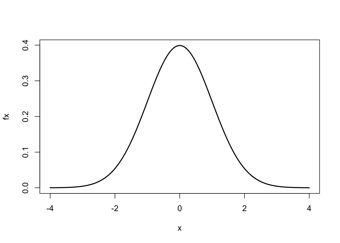

After assigning values to mu and sigma, we assigned to x a sequence of numbers from \(-4\) to 4 by intervals of 0.01. Using the normal curve equation, for every value of \(x\) we calculated \(f(x)\), represented by the numeric vector fx. We then used the plot function to plot \(x\) vs. \(f(x)\). The optional argument type='l' produces a ‘line’ and lwd=2 doubles the line width.

The rep function is used to replicate its arguments. Study the examples that follow:

rep(5, 2)           # repeat 5 2 times

## [1] 5 5

rep(1:2, 5)         # repeat 1:2 5 times

##  [1] 1 2 1 2 1 2 1 2 1 2

rep(1:2, c(5, 5))   # repeat 1 5 times; repeat 2 5 times

##  [1] 1 1 1 1 1 2 2 2 2 2

rep(1:2, rep(5, 2)) # equivalent to previous

##  [1] 1 1 1 1 1 2 2 2 2 2

rep(1:5, 5:1)       # repeat 1 5 times, repeat 2 4 times,...

##  [1] 1 1 1 1 1 2 2 2 2 3 3 3 4 4 5

The paste function pastes character strings:

fname <- c('John', 'Kenneth', 'Sander')
lname <- c('Snow', 'Rothman', 'Greenland')
paste(fname, lname)

## [1] "John Snow"        "Kenneth Rothman"  "Sander Greenland"

paste('var', 1:7, sep='')

## [1] "var1" "var2" "var3" "var4" "var5" "var6" "var7"

Indexing (subsetting) an object often results in a vector. To preserve the dimensionality of the original object use the drop option.

x <- matrix(1:8, 2, 4); x

##      [,1] [,2] [,3] [,4]
## [1,]    1    3    5    7
## [2,]    2    4    6    8

x[2, ]                    # index 2nd row

## [1] 2 4 6 8

x[2, , drop = FALSE]      # index 2nd row; keep structure

##      [,1] [,2] [,3] [,4]
## [1,]    2    4    6    8

Up to now we have generated vectors of known numbers or character strings. On occasion we need to generate random numbers or draw a sample from a collection of elements. First, sampling from a vector returns a vector:

sample(c('H', 'T'), size = 8, replace = T) # toss coin 8 times

## [1] "T" "H" "H" "T" "T" "T" "T" "H"

sample(1:6, size = 10, replace = TRUE) # toss die 10 times

##  [1] 2 4 6 4 5 1 2 2 4 6

Second, generating random numbers from a probability distribution returns a vector:

rbinom(n = 10, size = 50, p = 0.5)  # toss 50 coins 10 times

##  [1] 25 22 23 19 18 19 26 25 26 26

rnorm(5)  # generate 5 standard normal distribution values

## [1]  2.28897730 -0.03745504 -0.36735103  1.20308863  0.93610842

There are additional ways to create vectors. To practice creating vectors study the examples in Table 2.5 and spend a few minutes creating simple vectors. If we need help with a function remember enter ?function_name or help(function_name).

Finally, notice that we can use vectors as arguments to functions:

sample(c('head', 'tail'), 100, replace = TRUE)
rep(1:2, rep(5, 2))
matrix(c(23, 45, 16, 17), nrow = 2, ncol = 2)

2.2.3 Naming vectors

Each element of a vector can be labeled with a name at the time the vector is created or later. The first way of naming vector elements is when the vector is created:

x <- c(chol = 234, sbp = 148, dbp = 78, age = 54); x

## chol  sbp  dbp  age 
##  234  148   78   54

The second way is to create a character vector of names and then assign that vector to the numeric vector using the names function:

z <- c(234, 148, 78, 54); z

## [1] 234 148  78  54

names(z) <- c('chol', 'sbp', 'dbp', 'age'); z

## chol  sbp  dbp  age 
##  234  148   78   54

The names function, without an assignment, returns the character vector of names, if it exist. This character vector can be used to name elements of other vectors.

names(z)

## [1] "chol" "sbp"  "dbp"  "age"

z2 <- c(250, 184, 90, 45); z2

## [1] 250 184  90  45

names(z2) <- names(z); z2

## chol  sbp  dbp  age 
##  250  184   90   45

The unname function removes the element names from a vector:

unname(z2)

## [1] 250 184  90  45

For practice study the examples in Table 2.6 and spend a few minutes creating and naming simple vectors.

Table 2.6: Common ways of naming vectors

Function	Description	Try these examples
c	Name vector elements when vector is created	x <- c(a = 1, b = 2, c = 3, d = 4); x
names	Name vector elements	y <- 1:4; y
		names(y) <- c('a', 'b', 'c', 'd'); y
		names(y) # return names, if they exist
unname	Remove names (if they exist)	y <- unname(y) # equivalent: names(y) <- NULL
		y

2.2.4 Indexing vectors

Indexing a vector is subsetting or extracting elements from a vector. A vector is indexed by position, by name (if it exist), or by logical value (TRUE vs FALSE). Positions are specified by positive or negative integers.

x <- c(chol = 234, sbp = 148, dbp = 78, age = 54)
x[c(2, 4)]   # extract 2nd and 4th element

## sbp age 
## 148  54

x[-c(2, 4)]  # exclude 2nd and 4th element

## chol  dbp 
##  234   78

Although indexing by position is concise, indexing by name (when the names exists) is better practice in terms of documenting our code. Here is an example:

x[c('sbp', 'age')]  # extract 2nd and 4th element

## sbp age 
## 148  54

A logical vector indexes the positions that corresponds to the TRUEs. Here is an example:

x <= 100 | x > 200

##  chol   sbp   dbp   age 
##  TRUE FALSE  TRUE  TRUE

x[x <= 100 | x > 200]

## chol  dbp  age 
##  234   78   54

Any expression that evaluates to a valid vector of integers, names, or logicals can be used to index a vector.

(samp1 <- sample(1:4, 8, replace = TRUE))

## [1] 3 4 1 4 4 1 1 2

x[samp1]

##  dbp  age chol  age  age chol chol  sbp 
##   78   54  234   54   54  234  234  148

(samp2 <- sample(names(x), 8, replace = TRUE))

## [1] "sbp"  "dbp"  "sbp"  "age"  "chol" "sbp"  "chol" "chol"

x[samp2]

##  sbp  dbp  sbp  age chol  sbp chol chol 
##  148   78  148   54  234  148  234  234

Notice that when we indexed by position or name we indexed the same position repeatly. This will not work with logical vectors. In the example that follows NA means ‘not available.’

(samp3 <- sample(c(TRUE, FALSE), 8, replace = TRUE))

## [1]  TRUE  TRUE FALSE FALSE FALSE  TRUE FALSE  TRUE

x[samp3]

## chol  sbp <NA> <NA> 
##  234  148   NA   NA

We have already seen that a vector can be indexed based on the characteristics of another vector.

kid <- c('Tomasito', 'Irene', 'Luisito', 'Angelita', 'Tomas')
age <- c(8, NA, 7, 4, NA)
age <= 7                    # produces logical vector

## [1] FALSE    NA  TRUE  TRUE    NA

kid[age <= 7]               # index 'kid' using 'age'

## [1] NA         "Luisito"  "Angelita" NA

kid[!is.na(age)]            # remove missing values

## [1] "Tomasito" "Luisito"  "Angelita"

kid[age<=7 & !is.na(age)]

## [1] "Luisito"  "Angelita"

In this example, NA represents missing data. The is.na function returns a logical vector with s at NA positions. To generate a logical vector to index values that are not missing use !is.na.

For practice study the examples in Table 2.7 and spend a few minutes creating, naming, and indexing simple vectors.

Table 2.7: Common ways of indexing vectors

Indexing	Try these examples
By position	x <- c(chol = 234, sbp = 148, dbp = 78)
	x[2] # positions to include
	x[c(2, 3)]
	x[-c(1, 3)] # positions to exclude
	x[which(x<100)]
By name (if exists)	x['sbp']
	x[c('sbp', 'dbp')]
By logical	x < 100
	x[x < 100]
	(x < 150) & (x > 70)
	bp <- (x < 150) & (x > 70)
	x[bp]
Unique values	samp <- sample(1:5, 25, replace = TRUE)
	unique(samp)
Duplicated values	duplicated(samp) # generates logical
	samp[duplicated(samp)]

2.2.4.1 The which function

A Boolean operation that returns a logical vector contains TRUE values where the condition is true. To identify the position of each TRUE value we use the which function. For example, using the same data above:

which(age <= 7)        # which positions meet condition

## [1] 3 4

kid[which(age <= 7)]

## [1] "Luisito"  "Angelita"

Notice that is was unnecessary to remove the missing values.

2.2.5 Replacing vector elements (by indexing and assignment)

If a vector element can be indexed, it can be replaced. Therefore, to replace vector elements we combine indexing and assignment. Any elements of a vector that can be indexed can be replaced. Replacing vector elements is one method of recoding a variable. In this example, we recode a vector of ages into age categories:

age <- sample(0:100, 1000, replace = TRUE) # create vector
agecat <- age # copy vector
agecat[age<15] <- '<15'
agecat[age>=15 & age<25] <- '15-24'
agecat[age>=25 & age<45] <- '25-44'
agecat[age>=45 & age<65] <- '45-64'
agecat[age>=65] <- '65+'
table(agecat)

## agecat
##   <15 15-24 25-44 45-64   65+ 
##   159   114   217   196   314

First, we made a copy of the numeric vector age and named it agecat. Then, we replaced elements of agecat with character strings for each age category, creating a character vector.

For practice study the examples in Table 2.8 and spend a few minutes replacing vector elements.

Table 2.8: Common ways of replacing vector elements

Replacing	Try these examples
By position	x <- c(chol = 234, sbp = 148, dbp = 78)
	x[1]
	x[1] <- 250; x
By name (if exists)	x['sbp']
	x['sbp'] <- 150; x
By logical	x[x<100]
	x[x<100] <- NA; x

2.2.6 Operating on vectors Operating on vectors is very common in epidemiology and statistics.

In this section we cover common operations on single vectors (Table 2.9) and multiple vectors (Table 2.10).

2.2.6.1 Operating on single vectors

Table 2.9: Selected operations on single vectors

Function	Description		Function	Description
sum	summation		range	range
cumsum	cumulative sum		rev	reverse order
diff	x[i+1]-x[i]		order	order
prod	product		sort	sort
cumprod	cumulative product		rank	rank
mean	mean		sample	random sample
median	median		quantile	percentile
min	minimum		var	variance, covariance
max	maximum		sd	standard deviation

First, we focus on operating on single numeric vectors (Table 2.9). This also gives us the opportunity to see how common mathematical notation is translated into simple R code.

To sum elements of a numeric vector \(x\) of length \(n\), (\(\sum_{i=1}^{n}{x_i}\)), use the sum function:

x <- rnorm(100) # generate random standard normal values
sum(x)

## [1] -8.894035

To calculate a cumulative sum of a numeric vector \(x\) of length \(n\), (\(\sum_{i=1}^{k}{x_i}\), for \(k=1,\ldots,n\)), use the cumsum function which returns a vector:

x <- rep(2, 10); x # generate sequence of 2's; calculate cumulative sum

##  [1] 2 2 2 2 2 2 2 2 2 2

cumsum(x)

##  [1]  2  4  6  8 10 12 14 16 18 20

To multiply elements of a numeric vector \(x\) of length \(n\), (\(\prod_{i=1}^{n}{x_i}\)), use the prod function:

x <- c(1, 2, 3, 4, 5, 6, 7, 8)
prod(x)

## [1] 40320

To calculate the cumulative product of a numeric vector \(x\) of length \(n\), (\(\prod_{i=1}^{k}{x_i}\), for \(k=1,\ldots,n\)), use the cumprod function:

x <- c(1, 2, 3, 4, 5, 6, 7, 8)
cumprod(x)

## [1]     1     2     6    24   120   720  5040 40320

To calculate the mean of a numeric vector \(x\) of length \(n\), (\(\frac{1}{n} \sum_{i=1}^{n}{x_i}\)), use the sum and length functions, or use the mean function:

x <- rnorm(100)
sum(x)/length(x)

## [1] 0.1444784

mean(x)

## [1] 0.1444784

To calculate the sample variance of a numeric vector \(x\) of length \(n\), use the sum, mean, and length functions, or, more directly, use the var function.

\[\begin{equation} S_X^2 = \frac{1}{n-1} \left[ \sum_{i = 1}^n{(x_i - \bar{x})^2} \right] \end{equation}\]

x <- rnorm(100)
sum((x-mean(x))^2)/(length(x)-1)

## [1] 1.1538

var(x)  # equivalent

## [1] 1.1538

This example illustrates how we can implement a formula in R using several functions that operate on single vectors (sum, mean, and length). The var function, while available for convenience, is not necessary to calculate the sample variance.

When the var function is applied to two numeric vectors, \(x\) and \(y\), both of length \(n\), the sample covariance is calculated:

\[\begin{equation} S_{XY} = \frac{1}{n-1} \left[ \sum_{i = 1}^n{(x_i - \bar{x}) (y_i - \bar{y})} \right] \end{equation}\]

x <- rnorm(100); y <- rnorm(100)
sum((x - mean(x)) * (y - mean(y)))/(length(x) - 1)

## [1] -0.0935714

var(x, y)  # equivalent

## [1] -0.0935714

The sample standard deviation, of course, is just the square root of the sample variance (or use the sd function):

\[\begin{equation} S_X = \sqrt{\frac{1}{n-1} \left[ \sum_{i = 1}^n{(x_i - \bar{x})^2} \right]} \end{equation}\]

sqrt(var(x))

## [1] 0.9485411

sd(x)

## [1] 0.9485411

To sort a numeric or character vector use the sort function.

ages <- c(8, 4, 7)
sort(ages)

## [1] 4 7 8

However, to sort one vector based on the ordering of another vector use the order function.

ages <- c(8, 4, 7)
subjects <- c('Tomas', 'Angela', 'Luis')
subjects[order(ages)]

## [1] "Angela" "Luis"   "Tomas"

order(ages) # 'order' returns positional integers for sorting

## [1] 2 3 1

Notice that the order function does not return the data, but rather indexing integers in new positions for sorting the vector age or another vector. For example, order(ages) returned the integer vector c(2, 3, 1) which means ‘move the 2nd element ($ age = 4 \() to the first position, move the 3rd element (\)age = 7\() to the second position, and move the 1st element (\)age = 8$) to the third position.’ Verify that sort(ages) and ages[order(ages)] are equivalent.

To sort a vector in reverse order combine the rev and sort functions.

x <- c(12, 3, 14, 3, 5, 1)
sort(x)

## [1]  1  3  3  5 12 14

rev(sort(x))

## [1] 14 12  5  3  3  1

In contrast to the sort function, the rank function gives each element of a vector a rank score but does not sort the vector.

x <- c(12, 3, 14, 3, 5, 1)
rank(x)

## [1] 5.0 2.5 6.0 2.5 4.0 1.0

The median of a numeric vector is that value which puts 50% of the values below and 50% of the values above, in other words, the 50% percentile (or 0.5 quantile). For example, the median of c(4, 3, 1, 2, 5) is 3. For a vector of even length, the middle values are averaged: the median of c(4, 3, 1, 2) is 2.5. To get the median value of a numeric vector use the median or quantile function.

ages <- c(23, 45, 67, 33, 20, 77)
median(ages)

## [1] 39

quantile(ages, 0.5)

## 50% 
##  39

To return the minimum value of a vector use the min function; for the maximum value use the max function. To get both the minimum and maximum values use the range function.

ages <- c(23, 45, 67, 33, 20, 77)
min(ages)

## [1] 20

sort(ages)[1]  # equivalent

## [1] 20

max(ages)

## [1] 77

sort(ages)[length(ages)]  # equivalent

## [1] 77

range(ages)

## [1] 20 77

c(min(ages), max(ages))  # equivalent

## [1] 20 77

To sample from a vector of length \(n\), with each element having a default sampling probability of \(1/n\), use the sample function. Sampling can be with or without replacement (default). If the sample size is greater than the length of the vector, then sampling must occur with replacement.

coin <- c("H", "T")
sample(coin, size = 10, replace = TRUE)

##  [1] "T" "T" "H" "H" "T" "H" "T" "T" "T" "T"

sample(1:100, 15)

##  [1]  7 53 58 70 74 41 94 39 26 25 18 91 49 86 38

2.2.6.2 Operating on multiple vectors

Table 2.10: Selected operations on multiple vectors

Function	Description
c	Concatenates into vectors
append	Appends a vector to another vector
cbind	Column-bind vectors or matrices
rbind	Row-bind vectors or matrices
table	Creates contingency table from 2 or more vectors
xtabs	Creates contingency table from 2 or more factors in a data frame
ftable	Creates flat contingency table from 2 or more vectors
outer	Outer product
tapply	Applies a function to strata of a vector
<, >, <=, >=, ==, !=	Relational operators
!, |, xor	Logical operators

Next, we review selected functions that work with one or more vectors. Some of these functions manipulate vectors and others facilitate numerical operations.

In addition to creating vectors, the c function can be used to append vectors.

x <- 6:10
y <- 20:24
c(x, y)

##  [1]  6  7  8  9 10 20 21 22 23 24

The append function also appends vectors; however, one can specify at which position.

append(x, y)

##  [1]  6  7  8  9 10 20 21 22 23 24

append(x, y, after = 2)

##  [1]  6  7 20 21 22 23 24  8  9 10

In contrast, the cbind and rbind functions concatenate vectors into a matrix. During the outbreak of severe acute respiratory syndrome (SARS) in 2003, a patient with SARS potentially exposed 111 passengers on board an airline flight. Of the 23 passengers that sat ‘close’ to the index case, 8 developed SARS; among the 88 passengers that did not sit ‘close’ to the index case, only 10 developed SARS [@Olsen2003_pmid14681507]. Now, we can bind 2 vectors to create a \(2 \times 2\) table (matrix).

case <- c(exposed = 8, unexposed = 10)
noncase <- c(exposed = 15, unexposed = 78)
cbind(case, noncase)

##           case noncase
## exposed      8      15
## unexposed   10      78

rbind(case, noncase)

##         exposed unexposed
## case          8        10
## noncase      15        78

For the example that follows, let’s recreate the SARS data as two character vectors.

outcome <- c(rep("case", 8 + 10), rep("noncase", 15 + 78))
tmp <- c("exposed", "unexposed")
exposure <- c(rep(tmp, c(8, 10)), rep(tmp, c(15, 78)))
cbind(exposure, outcome)[1:4, ]  # display 4 rows

##      exposure  outcome
## [1,] "exposed" "case" 
## [2,] "exposed" "case" 
## [3,] "exposed" "case" 
## [4,] "exposed" "case"

Now, use the table function to cross-tabulate one or more vectors.

table(outcome, exposure)

##          exposure
## outcome   exposed unexposed
##   case          8        10
##   noncase      15        78

The ftable function creates a flat contingency table from one or more vectors.

ftable(outcome, exposure)

##         exposure exposed unexposed
## outcome                           
## case                   8        10
## noncase               15        78

This will come in handy later when we want to display a 3 or more dimensional table as a ‘flat’ 2-dimensional table.

The outer function applies a function to every combination of elements from two vectors. For example, create a multiplication table for the numbers 1 to 5.

outer(1:5, 1:5, '*')

##      [,1] [,2] [,3] [,4] [,5]
## [1,]    1    2    3    4    5
## [2,]    2    4    6    8   10
## [3,]    3    6    9   12   15
## [4,]    4    8   12   16   20
## [5,]    5   10   15   20   25

%% TODO %% NEED BETTER EXAMPLE HERE; POSSIBLY 3-D PLOT %% ?FRACTION TO VACCINATE VS. R0 AND VACCINE EFFICACY

The tapply function applies a function to strata of a vector that is defined by one or more ‘indexing’ vectors. For example, to calculate the mean age of females and males:

age <- c(23, 45, 67, 88, 22, 34, 80, 55, 21, 48)
sex <- c("M", "F", "M", "F", "M", "F", "M", "F", "M", "F")
tapply(X = age, INDEX = sex, FUN = mean)

##    F    M 
## 54.0 42.6

tapply(age, sex, sum)/tapply(age, sex, length)  # equivalent using tapply twice

##    F    M 
## 54.0 42.6

The tapply function is an important and versatile function because it allows us to apply any function that can be applied to a vector, to be applied to strata of a vector. Moveover, we can use our user-created functions as well.

2.3 A matrix is a 2-dimensional table of like elements

2.3.1 Understanding matrices

A matrix is a 2-dimensional table of like elements. Matrix elements can be either numeric, character, or logical. Contingency tables in epidemiology are represented in R as numeric matrices or arrays. An array is the generalization of matrices to 3 or more dimensions (commonly known as stratified tables). We cover arrays later, for now we will focus on 2-dimensional tables.

Consider the \(2\times 2\) table of crude data in Table 2.11 (Rothman 2012). In this randomized clinical trial (RCT), diabetic subjects were randomly assigned to receive either tolbutamide, an oral hypoglycemic drug, or placebo. Because this was a prospective study we can calculate risks, odds, a risk ratio, and an odds ratio. We will do this using R as a calculator.

Table 2.11: Deaths among subjects who received tolbutamide and placebo in the Unversity Group Diabetes Program (1970)

	Treatment
Outcome status	Tolbutamide	Placebo
Deaths	30	21
Survivors	174	184

dat <- matrix(c(30, 174, 21, 184), 2, 2)
rownames(dat) <- c('Deaths', 'Survivors')
colnames(dat) <- c('Tolbutamide', 'Placebo')
coltot <- apply(dat, 2, sum)   #column totals
risks <- dat['Deaths', ]/coltot
risk.ratio <- risks/risks[2]   #risk ratio
odds <- risks/(1 - risks)
odds.ratio <- odds/odds[2]     #odds ratio
dat                            # display results

##           Tolbutamide Placebo
## Deaths             30      21
## Survivors         174     184

rbind(risks, risk.ratio, odds, odds.ratio)

##            Tolbutamide   Placebo
## risks        0.1470588 0.1024390
## risk.ratio   1.4355742 1.0000000
## odds         0.1724138 0.1141304
## odds.ratio   1.5106732 1.0000000

Now let’s review each line briefly to understand the analysis in more detail.

rownames(dat) <- c('Deaths', 'Survivors')
colnames(dat) <- c('Tolbutamide', 'Placebo')

We used the rownames and the colnames functions to assign row and column names to the matrix dat. The row names and the column names are both character vectors.

coltot <- apply(dat, 2, sum)   #column totals

We used the apply function to sum the columns; it is a versatile function for applying any function to matrices or arrays. The second argument is the MARGIN option: in this case, MARGIN=2, meaning apply the sum function to the columns. To sum the rows, set MARGIN=1.

odds <- risks/(1-risks)
odds.ratio <- odds/odds[2]     #odds ratio

Using the definition of the odds, we calculated the odds of death for each treatment group. Then we calculated the odds ratios using the placebo group as the reference.

dat
rbind(risks, risk.ratio, odds, odds.ratio)

Finally, we display the dat table we created. We also created a table of results by row binding the vectors using the rbind function.

In the sections that follow we will cover the necessary concepts to make the previous analysis routine.

2.3.2 Creating matrices

%% Creating matrices

There are several ways to create matrices (Table 2.12). In general, we create or use matrices in the following ways:

• Contingency tables (cross tabulations)
• Spreadsheet calculations and display
• Collecting results into tabular form
• Results of 2-variable equations

Table 2.12: Common ways of creating a matrix

Function	Description	Try these examples
cbind	Column-bind vectors or matrices	x <- 1:3
		y <- 3:1
		z <- cbind(x, y); z
rbind	Row-bind vectors or matrices	z2 <- rbind(x, y); z2
matrix	Generates matrix	matrix(1:4, nrow=2, ncol=2)
dim	Assign dimensions to a data object	mtx2 <- 1:4; mtx2
		dim(mtx2) <- c(2, 2); mtx2
array	Generates matrix when array is 2-D	array(1:4, dim = c(2, 2))
table	Creates contingency table	table(infert$educ, infert$case)
xtabs	Creates contingency table using formula interface	xtabs(~education + case, data = infert)
ftable	Creates flat contingency table	ftable(infert$educ, infert$spont, infert$case)
as.matrix	Coerces object into a matrix	1:3
		as.matrix(1:3)
outer	Outer product of two vectors	outer(1:5, 1:5, '*')
x[row, , ]	Indexing an array can return a matrix	x <- array(1:8, c(2, 2, 2))
x[ ,col, ]		x[1, , ]
x[ , ,dep]		x[ ,1, ]
		x[ , ,1]

2.3.2.1 Contingency tables (cross tabulations)

In the previous section we used the matrix function to create the \(2 \times 2\) table for the UGDP clinical trial:

dat <- matrix(c(30, 174, 21, 184), 2, 2)
rownames(dat) <- c('Deaths', 'Survivors')
colnames(dat) <- c('Tolbutamide', 'Placebo'); dat

##           Tolbutamide Placebo
## Deaths             30      21
## Survivors         174     184

Alternatively, we can create a 2-way contingency table using the table function with fields from a data set;

dat2 <- read.table('~/git/phds/data/ugdp.txt', header = TRUE, sep = ',')
names(dat2) # display field names

## [1] "Status"    "Treatment" "Agegrp"

table(dat2$Status, dat2$Treatment)

##           
##            Placebo Tolbutamide
##   Death         21          30
##   Survivor     184         174

Alternatively, the xtabs function cross tabulates using a formula interface. An advantage of this function is that the field names are included.

xtabs(~Status + Treatment, data = dat2)

##           Treatment
## Status     Placebo Tolbutamide
##   Death         21          30
##   Survivor     184         174

Finally, a multi-dimensional contingency table can be presented as a 2-dimensional flat contingency table using the ftable function. Here we stratify the above table by the variable Agegrp.

xtab3way <- xtabs(~Status + Treatment + Agegrp, data=dat2)
xtab3way # xtabs produces an array

## , , Agegrp = <55
## 
##           Treatment
## Status     Placebo Tolbutamide
##   Death          5           8
##   Survivor     115          98
## 
## , , Agegrp = 55+
## 
##           Treatment
## Status     Placebo Tolbutamide
##   Death         16          22
##   Survivor      69          76

ftable(xtab3way) # convert to flat table

##                      Agegrp <55 55+
## Status   Treatment                 
## Death    Placebo              5  16
##          Tolbutamide          8  22
## Survivor Placebo            115  69
##          Tolbutamide         98  76

However, notice that ftable, while preserving the order of the variables, does provide the equivalent, namely, Status vs. Treatment, by Agegrp. We can fix this by reversing the order of the variables within the xtabs function:

ftable(xtabs(~Agegrp + Status + Treatment, data=dat2))

##                 Treatment Placebo Tolbutamide
## Agegrp Status                                
## <55    Death                    5           8
##        Survivor               115          98
## 55+    Death                   16          22
##        Survivor                69          76

%%% TODO create exercise about structure of ftable

2.3.2.2 Spreadsheet calculations and display

Matrices are commonly used to display spreadsheet-like calculations. In fact, a very efficient way to learn R is to use it as our spreadsheet. For example, assuming the rate of seasonal influenza infection is 10 infections per 100 person-years, let’s calculate the individual cumulative risk of influenza infection at the end of 1, 5, and 10 years. Assuming no competing risk, we can use the exponential formula:

\[\begin{equation} R(0, t) = 1 - e^{-\lambda t} \end{equation}\]

where , \(\lambda\) = infection rate, and \(t\) = time.

lamb <- 10/100
years <- c(1, 5, 10)
risk <- 1 - exp(-lamb*years)
cbind(rate = lamb, years, cumulative.risk = risk) # display

##      rate years cumulative.risk
## [1,]  0.1     1      0.09516258
## [2,]  0.1     5      0.39346934
## [3,]  0.1    10      0.63212056

Therefore, the cumulative risk of influenza infection after 1, 5, and 10 years is 9.5%, 39%, and 63%, respectively.

2.3.2.3 Collecting results into tabular form

A 2-way contingency table from the table or xtabs functions does not have margin totals. However, we can construct a numeric matrix that includes the totals. Using the UGDP data again,

dat2 <- read.table('~/git/phds/data/ugdp.txt', header = TRUE, sep = ',') 
tab2 <- xtabs(~Status + Treatment, data = dat2)
rowt <- tab2[, 1] + tab2[, 2]
tab2a <- cbind(tab2, Total = rowt)
colt <- tab2a[1, ] + tab2a[2, ]
tab2b <- rbind(tab2a, Total = colt)
tab2b

##          Placebo Tolbutamide Total
## Death         21          30    51
## Survivor     184         174   358
## Total        205         204   409

This table (tab2b) is primarily for display purposes.

2.3.2.4 Results of 2-variable equations

When we have an equation with 2 variables, we can use a matrix to display the answers for every combination of values contained in both variables. For example, consider this equation:

\[\begin{equation} z = x y \end{equation}\]

And suppose $ x = {1, 2, 3, 4, 5 } $ and $ y = {6, 7, 8, 9, 10 } $.

Here’s the long way to create a matrix for this equation:

x <- 1:5; y <- 6:10
z <- matrix(NA, 5, 5) #create empty matrix of missing values
for(i in 1:5){
    for(j in 1:5){
        z[i, j] <- x[i]*y[j]
    }
}
rownames(z) <- x; colnames(z) <- y; z

##    6  7  8  9 10
## 1  6  7  8  9 10
## 2 12 14 16 18 20
## 3 18 21 24 27 30
## 4 24 28 32 36 40
## 5 30 35 40 45 50

Okay, but the outer function is much better for this task:

x <- 1:5; y <- 6:10
z <- outer(x, y, '*')
rownames(z) <- x; colnames(z) <- y
z

##    6  7  8  9 10
## 1  6  7  8  9 10
## 2 12 14 16 18 20
## 3 18 21 24 27 30
## 4 24 28 32 36 40
## 5 30 35 40 45 50

In fact, the outer function can be used to calculate the ‘surface’ for any 2-variable equation (more on this later).

2.3.3 Naming matrix components

%% Jewell 2004, p. 83

We have already seen several examples of naming components of a matrix. Table 2.13 summarizes the common ways of naming matrix components. The components of a matrix can be named at the time the matrix is created, or they can be named later. For a matrix, we can provide the row names, column names, and field names.

Table 2.13: Common ways of naming matrix components

Function	Try these examples
matrix	# name rows and columns only
	dat <- matrix(c(178, 79, 1411, 1486), 2, 2,
	dimnames = list(c('Type A', 'Type B'), c('Yes', 'No')))
	# name rows, columns, and fields
	dat <- matrix(c(178, 79, 1411, 1486), 2, 2,
	dimnames = list(Behavior = c('Type A', 'Type B'),
	'Heart attack' = c('Yes', 'No')))
rownames	dat <- matrix(c(178, 79, 1411, 1486), 2, 2)
	rownames(dat) <- c('Type A', 'Type B')
colnames	colnames(dat) <- c('Yes', 'No') # col names
dimnames	# name rows and columns only
	dat <- matrix(c(178, 79, 1411, 1486), 2, 2)
	dimnames(dat) <- list(c('Type A', 'Type B'), c('Yes', 'No'))
	# name rows, columns, and fields
	dat <- matrix(c(178, 79, 1411, 1486), 2, 2)
	dimnames(dat) <- list(Behavior = c('Type A', 'Type B'),
	'Heart attack' = c('Yes', 'No'))
names	# add field to row \& col names
	`dat <- matrix(c(178, 79, 1411, 1486), 2, 2,
	dimnames = list(c('Type A', 'Type B'), c('Yes', 'No')))
	names(dimnames(dat)) <- c('Behavior', 'Heart attack')

For example, the UGDP clinical trial \(2 \times 2\) table can be created de novo:

ugdp2x2 <- matrix(c(30, 174, 21, 184), 2, 2, dimnames = list(Outcome = c('Deaths', 'Survivors'), 
                  Treatment = c('Tolbutamide', 'Placebo'))) 
ugdp2x2

##            Treatment
## Outcome     Tolbutamide Placebo
##   Deaths             30      21
##   Survivors         174     184

In the ‘Treatment’ field, the possible values, ‘Tolbutamide’ and ‘Placebo,’ are the column names. Similarly, in the ‘Status’ field, the possible values, ‘Death’ and ‘Survivor,’ are the row names.

If a matrix does not have field names, we can add them after the fact, but we must use the names and dimnames functions together. Having field names is necessary if the row and column names are not self-explanatory, as this example illustrates.

y <- matrix(c(30, 174, 21, 184), 2, 2)
rownames(y) <- c('Yes', 'No'); colnames(y) <- c('Yes', 'No')
y # labels not informative; add field names next

##     Yes  No
## Yes  30  21
## No  174 184

names(dimnames(y)) <- c('Death', 'Tolbutamide'); y

##      Tolbutamide
## Death Yes  No
##   Yes  30  21
##   No  174 184

Study and test the examples in Table 2.13.

2.3.4 Indexing a matrix

Similar to vectors, a matrix can be indexed by position, by name, or by logical. Study and practice the examples in (Table 2.14). An important skill to master is indexing rows of a matrix using logical vectors.

Table 2.14: Common ways of indexing a matrix

Indexing	Try these examples
By position	dat <- matrix(c(178, 79, 1411, 1486), 2, 2)
	dimnames(dat) <- list(Behavior = c('Type A', 'Type B'),
	'Heart attack' = c('Yes', 'No'))
	dat[1, ]
	dat[1,2]
	dat[2, , drop = FALSE]
By name (if exists)	dat['Type A', ]
	dat['Type A', 'Type B']
	dat['Type B', , drop = FALSE]
By logical	dat[, 1] > 100
	dat[dat[, 1] > 100, ]
	dat[dat[, 1] > 100, , drop = FALSE]

Consider the following matrix of data, and suppose I want to select the rows for subjects age less than 60 and systolic blood pressure less than 140.

age <- c(45, 56, 73, 44, 65)
chol <- c(145, 168, 240, 144, 210)
sbp <- c(124, 144, 150, 134, 112)
dat <- cbind(age, chol, sbp); dat

##      age chol sbp
## [1,]  45  145 124
## [2,]  56  168 144
## [3,]  73  240 150
## [4,]  44  144 134
## [5,]  65  210 112

dat[, 'age'] < 60

## [1]  TRUE  TRUE FALSE  TRUE FALSE

dat[, 'sbp'] < 140

## [1]  TRUE FALSE FALSE  TRUE  TRUE

tmp <- dat[, 'age'] < 60 & dat[, 'sbp'] < 140; tmp

## [1]  TRUE FALSE FALSE  TRUE FALSE

dat[tmp, ] # index rows using logical vector 'tmp'

##      age chol sbp
## [1,]  45  145 124
## [2,]  44  144 134

Notice that the tmp logical vector is the intersection of the logical vectors separated by the logical operator &.

2.3.5 Replacing matrix elements

Remember, replacing matrix elements is just indexing plus assignment: anything that can be indexed can be replaced. Study and practice the examples in (Table 2.15).

Table 2.15: Common ways of replacing matrix elements

Replacing	Try these examples
By position	dat <- matrix(c(178, 79, 1411, 1486), 2, 2)
	dimnames(dat) <- list(c('Type A','Type B'), c('Yes','No'))
	dat[1, ] <- 99; dat
By name (if exists)	dat['Type A', ] <- c(178, 1411); dat
By logical	qq <- dat[, 1] < 100 # logic vector
	dat[qq, ] <- 99; dat
	dat[dat[, 1] < 100, ] <- c(79, 1486); dat

2.3.6 Operating on a matrix

In epidemiology books, authors have preferences for displaying contingency tables. Software packages have default displays for contingency tables. In practice, we may need to manipulate a contingency table to facilitate further analysis. Consider the following 2-way table:

tab <- matrix(c(30, 174, 21, 184), 2, 2, dimnames = list(Outcome = c('Deaths', 'Survivors'), 
             Treatment = c('Tolbutamide', 'Placebo'))); tab

##            Treatment
## Outcome     Tolbutamide Placebo
##   Deaths             30      21
##   Survivors         174     184

We can transpose the matrix using the t function.

t(tab)

##              Outcome
## Treatment     Deaths Survivors
##   Tolbutamide     30       174
##   Placebo         21       184

We can reverse the order of the rows and/or columns.

tab[2:1, ]               # reverse rows

##            Treatment
## Outcome     Tolbutamide Placebo
##   Survivors         174     184
##   Deaths             30      21

tab[,2:1]                # reverse columns

##            Treatment
## Outcome     Placebo Tolbutamide
##   Deaths         21          30
##   Survivors     184         174

tab[2:1, 2:1]            # reverse rows and columns

##            Treatment
## Outcome     Placebo Tolbutamide
##   Survivors     184         174
##   Deaths         21          30

In short, we need to be able to manipulate and execute operations on a matrix. Table 2.16 summarizes key functions (apply and sweep) for passing other functions to execute operations on a matrix. Table 2.17 summarizes additional convenience functions for operating on a matrix.

Table 2.16: Common ways of operating on a matrix

Function	Description	Try these examples
t	Transpose matrix	dat <- matrix(c(178, 79, 1411, 1486), 2, 2)
		t(dat)
apply	Apply a function to margins of a matrix	apply(X = dat, MARGIN = 2, FUN = sum)
		apply(dat, 1, FUN=sum)
		apply(dat, 1, mean)
		apply(dat, 2, cumprod)
sweep	Sweeping out a summary statistic	rsum <- apply(dat, 1, sum)
		rdist <- sweep(dat, 1, rsum, '/')
		rdist
		csum <- apply(dat, 2, sum)
		cdist <- sweep(dat, 2, csum, '/')
		cdist

Table 2.17: Alternative ways of operating on a matrix (with equivalents)

Function	Description	Try these examples
margin.table,	For array tables, get marginals	dat <- matrix(5:8, 2, 2)
rowSums,		margin.table(dat)
colSums		margin.table(dat, 1)
		rowSums(dat) # equivalent
		apply(dat, 1, sum) # equivalent
		margin.table(dat, 2)
		colSums(dat) # equivalent
		apply(dat, 2, sum) # equivalent
addmargins	Marginal totals	addmargins(dat)
rowMeans,	For array tables, get marginal means	rowMeans(dat)
colMeans		apply(dat, 1, mean) # equivalent
		colMeans(dat)
		apply(dat, 2, mean) # equivalent
prop.table	For array tables, get marginal distributions	prop.table(dat)
		dat/sum(dat) # equivalent
		prop.table(dat, 1)
		sweep(dat, 1, apply(y,1,sum), '/')
		prop.table(dat, 2)
		sweep(y, 2, apply(y, 2, sum), '/')

2.3.6.1 The apply function

The apply function is an important and versatile function for conducting operations on rows or columns of a matrix, including user-created functions. The same functions that are used to conduct operations on single vectors (Table 2.9) can be applied to rows or columns of a matrix.

To calculate the row or column totals use the apply with the sum function:

tab

##            Treatment
## Outcome     Tolbutamide Placebo
##   Deaths             30      21
##   Survivors         174     184

apply(tab, 1, sum) # row totals

##    Deaths Survivors 
##        51       358

apply(tab, 2, sum) # column totals

## Tolbutamide     Placebo 
##         204         205

These operations can be used to calculate marginal totals and have them combined with the original table into one table.

tab

##            Treatment
## Outcome     Tolbutamide Placebo
##   Deaths             30      21
##   Survivors         174     184

rtot <- apply(tab, 1, sum)             # row totals
tab2 <- cbind(tab, Total = rtot); tab2

##           Tolbutamide Placebo Total
## Deaths             30      21    51
## Survivors         174     184   358

ctot <- apply(tab2, 2, sum)            # column totals
rbind(tab2, Total = ctot)

##           Tolbutamide Placebo Total
## Deaths             30      21    51
## Survivors         174     184   358
## Total             204     205   409

For convenience, R provides some functions for calculating marginal totals, and calculating row or column means (margin.table, rowSums, colSums, rowMeans, and colMeans). However, these functions just use the apply function.⁸

Here’s an alternative method to calculate marginal totals:

tab

##            Treatment
## Outcome     Tolbutamide Placebo
##   Deaths             30      21
##   Survivors         174     184

tab2 <- cbind(tab, Total = rowSums(tab))
rbind(tab2, Total = colSums(tab2))

##           Tolbutamide Placebo Total
## Deaths             30      21    51
## Survivors         174     184   358
## Total             204     205   409

For convenience, the addmargins function calculates and displays the marginals totals with the original data in one step.

tab <- matrix(c(30, 174, 21, 184), 2, 2, dimnames = list(Outcome = c('Deaths', 'Survivors'), 
                  Treatment = c('Tolbutamide', 'Placebo')))
tab

##            Treatment
## Outcome     Tolbutamide Placebo
##   Deaths             30      21
##   Survivors         174     184

addmargins(tab)

##            Treatment
## Outcome     Tolbutamide Placebo Sum
##   Deaths             30      21  51
##   Survivors         174     184 358
##   Sum               204     205 409

The power of the apply function comes from our ability to pass many functions (including our own) to it. For practice, combine the apply function with functions from Table 2.9 to conduct operations on rows and columns of a matrix.

2.3.6.2 The sweep function

The sweep function is another important and versatile function for conducting operations across rows or columns of a matrix. This function ‘sweeps’ (operates on) a row or column of a matrix using some function and a value (usually derived from the row or column values). To understand this, we consider an example involving a single vector. For a given integer vector x, to convert the values of x into proportions involves two steps:

x <- c(1, 2, 3, 4, 5)
sumx <- sum(x) # Step 1 summation
x/sumx         # Step 2 division (the 'sweep')

## [1] 0.06666667 0.13333333 0.20000000 0.26666667 0.33333333

To apply this equivalent operation across rows or columns of a matrix requires the sweep function.

For example, to calculate the row and column distributions of a 2-way table we combine the apply (step 1) and the sweep (step 2) functions:

tab

##            Treatment
## Outcome     Tolbutamide Placebo
##   Deaths             30      21
##   Survivors         174     184

rtot <- apply(tab, 1, sum)              # row totals
tab.rowdist <- sweep(tab, 1, rtot, '/'); tab.rowdist

##            Treatment
## Outcome     Tolbutamide   Placebo
##   Deaths      0.5882353 0.4117647
##   Survivors   0.4860335 0.5139665

ctot <- apply(tab, 2, sum)              # column totals
tab.coldist <- sweep(tab, 2, ctot, '/'); tab.coldist

##            Treatment
## Outcome     Tolbutamide  Placebo
##   Deaths      0.1470588 0.102439
##   Survivors   0.8529412 0.897561

Because R is a true programming language, these can be combined into single steps:

sweep(tab, 1, apply(tab, 1, sum), '/') #row distribution

##            Treatment
## Outcome     Tolbutamide   Placebo
##   Deaths      0.5882353 0.4117647
##   Survivors   0.4860335 0.5139665

sweep(tab, 2, apply(tab, 2, sum), '/') #column distribution

##            Treatment
## Outcome     Tolbutamide  Placebo
##   Deaths      0.1470588 0.102439
##   Survivors   0.8529412 0.897561

For convenience, R provides prop.table. However, this function just uses the apply and sweep functions.

%% TODO consider demo of prop.table

2.4 An array is a n-dimensional table of like elements

While a matrix is a 2-dimensional table of like elements, an array is the generalization of matrices to \(n\)-dimensions. Stratified contingency tables in epidemiology are represented as array data objects in R. For example, the randomized clinical trial previously shown comparing the number deaths among diabetic subjects that received tolbutamide vs. placebo is now also stratified by age group (Table 2.18):

2.4.1 Understanding arrays

Table 2.18: Deaths among subjects who received tolbutamide (TOLB) and placebo in the Unversity Group Diabetes Program (1970) stratifying by age

	Age<55			Age>=55			Combined
	TOLB	Placebo		TOLB	Placebo		TOLB	Placebo
Deaths	8	5		22	16		30	21
Survivors	98	115		76	69		174	184
Total	106	120		98	85		204	205

This is 3-dimensional array: outcome status vs. treatment status vs. age group. Let’s see how we can represent this data in R.

tdat <- c(8, 98, 5, 115, 22, 76, 16, 69)
tdat <- array(tdat, c(2, 2, 2))
dimnames(tdat) <- list(Outcome = c('Deaths', 'Survivors'), 
                    Treatment = c('Tolbutamide', 'Placebo'), 
                    'Age group' = c('Age<55', 'Age>=55')); tdat

## , , Age group = Age<55
## 
##            Treatment
## Outcome     Tolbutamide Placebo
##   Deaths              8       5
##   Survivors          98     115
## 
## , , Age group = Age>=55
## 
##            Treatment
## Outcome     Tolbutamide Placebo
##   Deaths             22      16
##   Survivors          76      69

R displays the first stratum (tdat[,,1]) then the second stratum (tdat[,,2]). Our goal now is to understand how to generate and operate on these types of arrays. Before we can do this we need to thoroughly understand the structure of arrays.

Let’s study a 4-dimensional array. Displayed in Table 2.19 is the year 2000 population estimates for Alameda and San Francisco Counties by age, ethnicity, and sex. The first dimension is age category, the second dimension is ethnicity, the third dimension is sex, and the fourth dimension is county. Learning how to visualize this 4-dimensional sturcture in R will enable us to visualize arrays of any number of dimensions.

Table 2.19: Year 2000 population estimates by age, ethnicity, sex, and county

County, Sex, & Age	White	Black	AsianPI	Latino	Multirace	AmerInd
Alameda Female, Age
<=19	58,160	31,765	40,653	49,738	10,120	839
20–44	112,326	44,437	72,923	58,553	7,658	1,401
45–64	82,205	24,948	33,236	18,534	2,922	822
65+	49,762	12,834	16,004	7,548	1,014	246
Alameda Male, Age
<=19	61,446	32,277	42,922	53,097	10,102	828
20–44	115,745	36,976	69,053	69,233	6,795	1,263
45–64	81,332	20,737	29,841	17,402	2,506	687
65+	33,994	8,087	11,855	5,416	711	156
SF Female, Age
<=$19	14355	6986	23265	13251	2940	173
20–44	85766	10284	52479	23458	3656	526
45–64	35617	6890	31478	9184	1144	282
65+	27215	5172	23044	5773	554	121
SF Male, Age
<=19	14881	6959	24541	14480	2851	165
20–44	105798	11111	48379	31605	3766	782
45–64	43694	7352	26404	8674	1220	354
65+	20072	3329	17190	3428	450	76

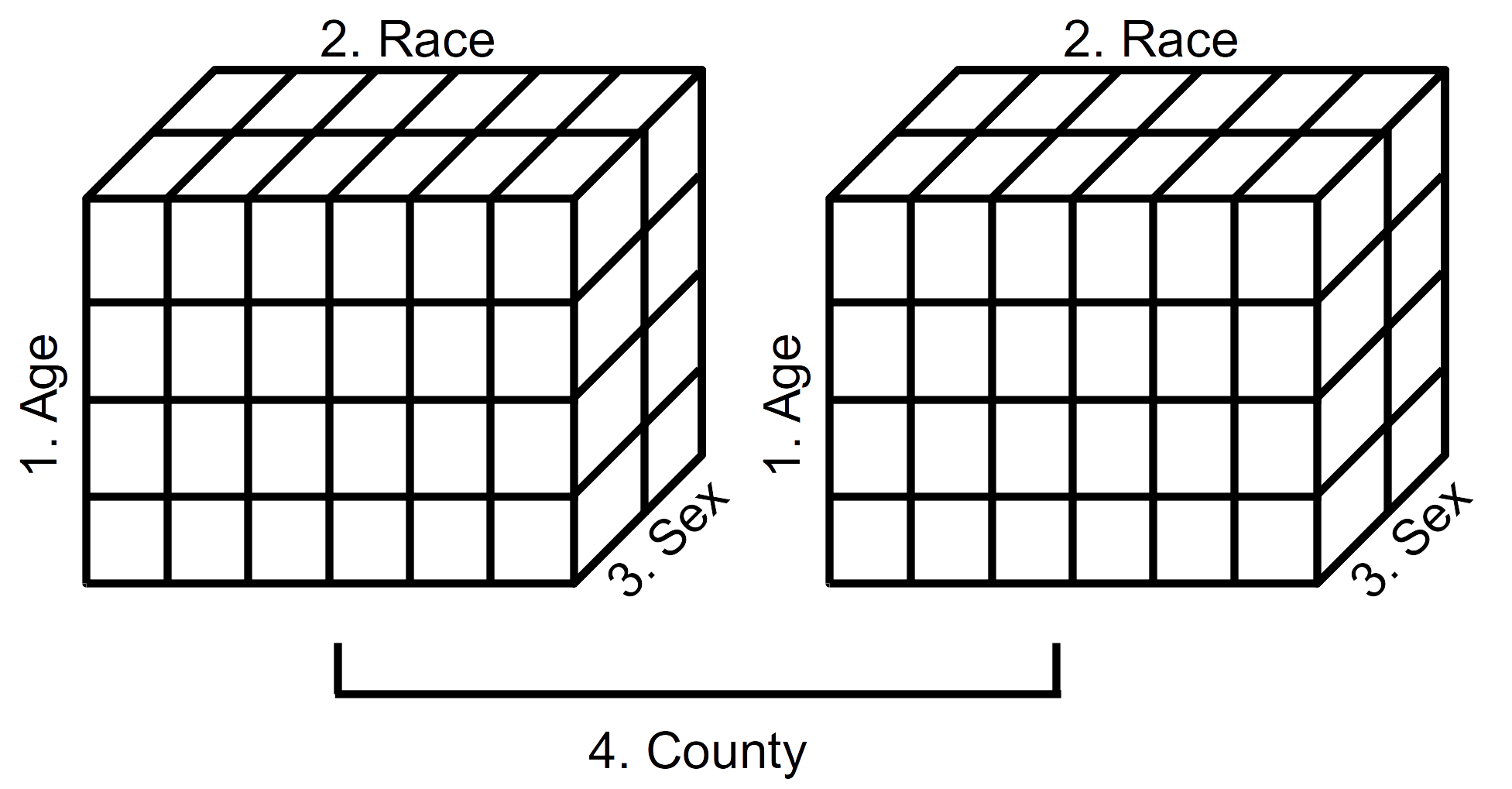
Figure 2.1: Schematic representation of a 4-dimensional array (Year 2000 population estimates by age, race, sex, and county)

Displayed in Figure 2.1 is a schematic representation of the 4-dimensional array of population estimates in Table 2.19. The left cube represents the population estimates by age, race, and sex (dimensions 1, 2, and 3) for Alameda County (first component of dimension 4). The right cube represents the population estimates by age, race, and sex (dimensions 1, 2, and 3) for San Francisco County (second component of dimension 4). We see, then, that it is possible to visualize data arrays in more than three dimensions.

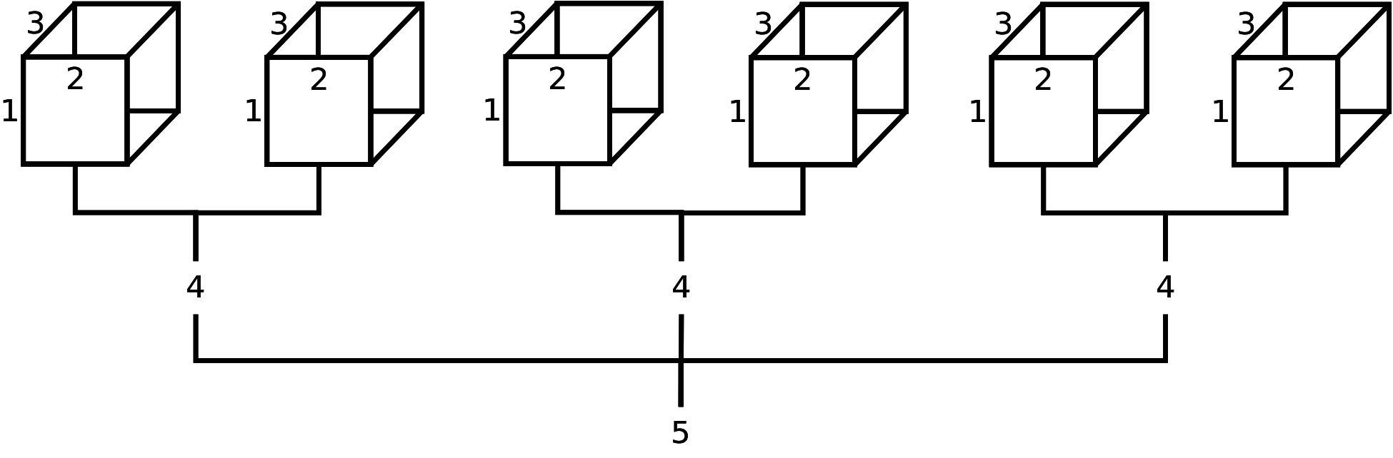
Figure 2.2: Schematic representation of a theoretical 5-dimensional array (possibly population estimates by age (1), race (2), sex (3), party affiliation (4), and state (5)). From this diagram, we can infer that the field ‘state’ has 3 levels, and the field ‘party affiliation’ has 2 levels; however, it is not apparent how many age levels, race levels, and sex levels have been created. Although not displayed, age levels would be represented by row names (along 1st dimension), race levels would be represented by column names (along 2nd dimension), and sex levels would be represented by depth names (along 3rd dimension).

To convince ourselves further, displayed in Figure 2.2 is a theorectical 5-dimensional data array. Suppose this 5-D array contained data on age (‘Young’, ‘Old’), ethnicity (‘White’, ‘Nonwhite’), sex (‘Male’, ‘Female’), party affiliation (‘Democrat’, ‘Republican’), and state (‘California’, ‘Washington State’, ‘Florida’). For practice, using fictitious data, try the following R code and study the output:

tab5 <- array(1:48, dim = c(2,2,2,2,3))
dn1 <- c('Young', 'Old')
dn2 <- c('White', 'Nonwhite')
dn3 <- c('Male', 'Female')
dn4 <- c('Democrat', 'Republican')
dn5 <- c('California', 'Washington State', 'Florida')
dimnames(tab5) <- list(Age = dn1, Race = dn2, Sex = dn3, Party=dn4, State=dn5)
tab5

2.4.2 Creating arrays

In R, arrays are most often produced with the array, table, or xtabs functions (Table 2.20). As in the previous example, the array function works much like the matrix function except the array function can specify 1 or more dimensions, and the matrix function only works with 2 dimensions.

array(1, dim = 1)

## [1] 1

array(1, dim = c(1, 1))

##      [,1]
## [1,]    1

array(1, dim = c(1, 1, 1))

## , , 1
## 
##      [,1]
## [1,]    1

Table 2.20: Common ways of creating arrays

Function	Description	Try these examples
array	Reshapes vector into an array	aa <- array(1:12, dim = c(2, 3, 2)); aa
table	Creates n-dimensional contingency table from n vectors	data(infert) # load infert data set
		table(infert$educ, infert$spont, infert$case)
xtabs	Creates a contingency table from data frames using formula interface	xtabs(\~{}education + case + parity, data = infert)
as.table	Creates n-dimensional contingency table from \(n\)-dimensional ftable	ft <- ftable(infert$educ, infert$spont, infert$case); ft
		as.table(ft)
dim	Assign dimensions to a data object	x <- 1:12; x
		dim(x) <- c(2, 3, 2); x

The table and xtabs functions cross tabulate two or more categorical vectors, except that xtabs only works with data frames. In R, categorical data are represented by character vectors or factors.⁹ First, we cross tabulate character vectors using table and xtabs.

 ## read data 'as is' (no factors created)
udat1 <- read.csv('~/git/phds/data/ugdp.txt', as.is = TRUE) 
str(udat1)

## 'data.frame':    409 obs. of  3 variables:
##  $ Status   : chr  "Death" "Death" "Death" "Death" ...
##  $ Treatment: chr  "Tolbutamide" "Tolbutamide" "Tolbutamide" "Tolbutamide" ...
##  $ Agegrp   : chr  "<55" "<55" "<55" "<55" ...

table(udat1$Status, udat1$Treatment, udat1$Agegrp)

## , ,  = <55
## 
##           
##            Placebo Tolbutamide
##   Death          5           8
##   Survivor     115          98
## 
## , ,  = 55+
## 
##           
##            Placebo Tolbutamide
##   Death         16          22
##   Survivor      69          76

The as~is option assured that character vectors were not converted to factors, which is the default. Notice that the table function produced an array with no field names (i.e., Status, Treatment, Agegrp). This is not ideal. A better option is to use xtabs, which uses a formula interface (~ V1 + V2):

xtabs(~ Status + Treatment + Agegrp, data = udat1)

## , , Agegrp = <55
## 
##           Treatment
## Status     Placebo Tolbutamide
##   Death          5           8
##   Survivor     115          98
## 
## , , Agegrp = 55+
## 
##           Treatment
## Status     Placebo Tolbutamide
##   Death         16          22
##   Survivor      69          76

Notice that xtabs includes the field names. For practice with cross tabulating factors, repeat the above expressions with read in the data setting option as is to FALSE.

Although table does not generate the field names, they can be added manually:

table(Outcome = udat1$Status, Therapy = udat1$Treatment, Age = udat1$Agegrp)

## , , Age = <55
## 
##           Therapy
## Outcome    Placebo Tolbutamide
##   Death          5           8
##   Survivor     115          98
## 
## , , Age = 55+
## 
##           Therapy
## Outcome    Placebo Tolbutamide
##   Death         16          22
##   Survivor      69          76

Recall that the ftable function creates a flat contingency from categorical vectors. The as.table function converts the flat contingency table back into a multidimensional array.

ftab <- ftable(Age = udat1$Agegrp, Therapy = udat1$Treatment, Outcome = udat1$Status); ftab

##                 Outcome Death Survivor
## Age Therapy                           
## <55 Placebo                 5      115
##     Tolbutamide             8       98
## 55+ Placebo                16       69
##     Tolbutamide            22       76

as.table(ftab) 

## , , Outcome = Death
## 
##      Therapy
## Age   Placebo Tolbutamide
##   <55       5           8
##   55+      16          22
## 
## , , Outcome = Survivor
## 
##      Therapy
## Age   Placebo Tolbutamide
##   <55     115          98
##   55+      69          76

2.4.3 Naming arrays

Naming components of an array is an extension of naming components of a matrix (Table 2.13). Study and implement the examples in Table 2.21.

%% Jewell 2004, p. 124

Table 2.21: Common ways of naming arrays

Function	Comments	Try these examples
array	Create labels for	x <- c(140, 11, 280, 56, 207, 9, 275, 32)
	values of each	rn <- c('>=1 cups per day', '0 cups per day')
	dimension	cn <- c('Cases', 'Controls')
		dn <- c('Females', 'Males')
		x <- array(x, dim = c(2, 2, 2),
		dimnames = list(Coffee = rn,
		Outcome = cn, Gender = dn)); x
dimnames	Create labels for	x <- c(140, 11, 280, 56, 207, 9, 275, 32)
	values of each	rn <- c('>=1 cups per day', '0 cups per day')
	dimension	cn <- c('Cases', 'Controls')
		dn <- c('Females', 'Males')
		x <- array(x, dim = c(2, 2, 2))
		dimnames(x) <- list(Coffee = rn, Outcome = cn,
		Gender = dn); x
names	Create labels for	x <- c(140, 11, 280, 56, 207, 9, 275, 32)
	values of each	rn <- c('>=1 cups per day', '0 cups per day')
	dimension	cn <- c('Cases', 'Controls')
		dn <- c('Females', 'Males')
		x <- array(x, dim = c(2, 2, 2))
		dimnames(x) <- list(rn, cn, dn)
		x # display w/o field names
		names(dimnames(x))<-c('Coffee', 'Case status', 'Sex')
		x # display w/ field names

2.4.4 Indexing arrays

Indexing an array is an extension of indexing a matrix (Table 2.14). Study and implement the examples in (Table 2.22).

Table 2.22: Common ways of indexing arrays

Indexing	Try these examples
By position	x[1, , ]
	x[ ,2 , ]
By name (if exists)	x[ , , 'Males']
	x[ ,'Controls', 'Females']
By logical vector	zz <- x[ ,1,1]>50; zz
	x[zz, , ]

2.4.5 Replacing array elements

Replacing elements of an array is an extension of replacing elements of a matrix (Table 2.15). Study and implement the examples in (Table 2.23).

Table 2.23: Common ways of replacing array elements

Replacing	Try these examples
By position	# use x from Table 2.21
	x[1, 1, 1] <- NA
	x
By name (if exists)	x[ ,'Controls', 'Females'] <- 99; x
By logical	x > 200
	x[x > 200] <- 999
	x

2.4.6 Operating on an array

With the exception of the aperm function, operating on an array (Table 2.24) is an extension of operating on a matrix (Table 2.16). The second group of functions, such as margin.table, are shortcuts provided for convenience. In other words, these operations are easily accomplished using apply and/or sweep.

%% x <- c(140, 11, 280, 56, 207, 9, 275, 32) %% x <- array(x, dim = c(2, 2, 2)) %% rn <- c(‘>=1 cups per day’, ‘0 cups per day’) %% cn <- c(‘Cases’, ‘Controls’) %% dn <- c(‘Females’, ‘Males’) %% dimnames(x) <- list(Coffee = rn, Outcome = cn, Gender = dn) %% x %% aperm(x, c(3, 2, 1))

Table 2.24: Common ways of operating on an array

Function	Description
aperm	Transpose an array by permuting its dimensions and optionally resizing it
apply	Apply a function to the margins of an array
sweep	Return an array obtained from an input array by sweeping out a summary statistic
	The following short-cuts use apply and/or sweep functions
margin.table	For a contingency table in array form, sum of table entries for a given index
rowSums	Sum across rows of an array
colSums	Sum down columns of an array
addmargins	Calculate and display marginal totals of an array
rowMeans	Calculate means across rows of an array
colMeans	Calculate means down columns of an array
prop.table	Generates distribution for dimensions that are summed in the margins

%%% TODO complete syphilis table 2013-10-30

Table 2.25: Example of 3-dimensional array with marginal totals: Primary and secondary syphilis morbidity by age, race, and sex, United State, 1989 (Source: CDC Summary of Notifiable Diseases, United States, 1989, MMWR 1989;38(54))

Age (yrs)	Sex	White	Black	Other	Total
<=19	Male	90	1,443	217	1,750
	Female	267	2,422	169	2,858
	Total	357	3,865	386	4,608
20–29	Male	957	8,180	1,287	10,424
	Female	908	8,093	590	9,591
	Total	1,865	16,273	1,877	20,015
30–44	Male	1,218	8,311	1,012	10,541
	Female	559	4,133	316	5,008
	Total	1,777	12,444	1,328	15,549
45+	Male	539	2,442	310	3,291
	Female	79	484	55	618
	Total	618	2,926	365	3,909
Total (by sex & ethnicity)	Male	2,804	20,376	2,826	26,006
	Female	1,813	15,132	1,130	18,075
Total (by ethnicity)		4617	35508	3956	44081

Consider the number of primary and secondary syphilis cases in the United State, 1989, stratified by sex, ethnicity, and age (Table 2.25). This table contains the marginal and joint distribution of cases. Let’s read in the original data and reproduce the table results.

sdat5 <- read.csv('~/git/phds/data/syphilis89d.txt')
str(sdat5) # structure of data frame

## 'data.frame':    44081 obs. of  3 variables:
##  $ Sex : Factor w/ 2 levels "Female","Male": 2 2 2 2 2 2 2 2 2 2 ...
##  $ Race: Factor w/ 3 levels "Black","Other",..: 3 3 3 3 3 3 3 3 3 3 ...
##  $ Age : Factor w/ 4 levels "<=19","20-29",..: 1 1 1 1 1 1 1 1 1 1 ...

lapply(sdat5, levels) # levels for each variable

## $Sex
## [1] "Female" "Male"  
## 
## $Race
## [1] "Black" "Other" "White"
## 
## $Age
## [1] "<=19"  "20-29" "30-44" "45+"

In R, categorical data are converted into factors. The possible values for each factor are called levels. We used lapply to pass the levels function and display the levels for each factor. In order to match the table display we need to reorder the levels for Sex and Race, and we recode Age into four levels.

sdat5$Sex <- factor(sdat5$Sex, levels = c('Male', 'Female'))
sdat5$Race <- factor(sdat5$Race, levels = c('White', 'Black', 'Other'))
lapply(sdat5, levels) # verify

## $Sex
## [1] "Male"   "Female"
## 
## $Race
## [1] "White" "Black" "Other"
## 
## $Age
## [1] "<=19"  "20-29" "30-44" "45+"

We used the factor function and the levels option to reorder the levels. Now we are ready to create an array and calculate the marginal totals to replicate Table 2.25.

sdat <- xtabs(~Sex+Race+Age, data=sdat5) # array
sdat

## , , Age = <=19
## 
##         Race
## Sex      White Black Other
##   Male      90  1443   217
##   Female   267  2422   169
## 
## , , Age = 20-29
## 
##         Race
## Sex      White Black Other
##   Male     957  8180  1287
##   Female   908  8093   590
## 
## , , Age = 30-44
## 
##         Race
## Sex      White Black Other
##   Male    1218  8311  1012
##   Female   559  4133   316
## 
## , , Age = 45+
## 
##         Race
## Sex      White Black Other
##   Male     539  2442   310
##   Female    79   484    55

To get marginal totals for one dimension, use the apply function and specify the dimension for stratifying the results.

sum(sdat) #total

## [1] 44081

apply(sdat, 1, sum) # by sex

##   Male Female 
##  26006  18075

apply(sdat, 2, sum) # by race

## White Black Other 
##  4617 35508  3956

apply(sdat, 3, sum) # by age

##  <=19 20-29 30-44   45+ 
##  4608 20015 15549  3909

To get the joint marginal totals for 2 or more dimensions, use the apply function and specify the dimensions for stratifying the results. This means that the function that is passed to apply is applied across the other, non-stratified dimensions.

apply(sdat, c(1, 2), sum) # by sex and race

##         Race
## Sex      White Black Other
##   Male    2804 20376  2826
##   Female  1813 15132  1130

apply(sdat, c(1, 3), sum) # by sex and age

##         Age
## Sex      <=19 20-29 30-44  45+
##   Male   1750 10424 10541 3291
##   Female 2858  9591  5008  618

apply(sdat, c(3, 2), sum) # by age and race

##        Race
## Age     White Black Other
##   <=19    357  3865   386
##   20-29  1865 16273  1877
##   30-44  1777 12444  1328
##   45+     618  2926   365

In R, arrays are displayed by the 1st and 2nd dimensions, stratified by the remaining dimensions. To change the order of the dimensions, and hence the display, use the aperm function. For example, the syphilis case data is most efficiently displayed when it is stratified by race, age, and sex:

sdat.ras <- aperm(sdat, c(2, 3, 1)); sdat.ras

## , , Sex = Male
## 
##        Age
## Race    <=19 20-29 30-44  45+
##   White   90   957  1218  539
##   Black 1443  8180  8311 2442
##   Other  217  1287  1012  310
## 
## , , Sex = Female
## 
##        Age
## Race    <=19 20-29 30-44  45+
##   White  267   908   559   79
##   Black 2422  8093  4133  484
##   Other  169   590   316   55

Using aperm we moved the 2nd dimension (race) into the first position, the 3rd dimension (age) into the second position, and the 1st dimension (sex) into the third position.

Another method for changing the display of an array is to convert it into a flat contingency table using the ftable function. For example, to display Table 2.25 as a flat contingency table in R (but without the marginal totals), we use the following code:

sdat.asr <- aperm(sdat, c(3,1,2)) # arrange age, sex, race
ftable(sdat.asr)                  # convert 2-D flat table

##              Race White Black Other
## Age   Sex                          
## <=19  Male           90  1443   217
##       Female        267  2422   169
## 20-29 Male          957  8180  1287
##       Female        908  8093   590
## 30-44 Male         1218  8311  1012
##       Female        559  4133   316
## 45+   Male          539  2442   310
##       Female         79   484    55

This ftable object can be treated as a matrix, but it cannot be transposed. Also, notice that we can combine the ftable with addmargins:

ftable(addmargins(sdat.asr))

##              Race White Black Other   Sum
## Age   Sex                                
## <=19  Male           90  1443   217  1750
##       Female        267  2422   169  2858
##       Sum           357  3865   386  4608
## 20-29 Male          957  8180  1287 10424
##       Female        908  8093   590  9591
##       Sum          1865 16273  1877 20015
## 30-44 Male         1218  8311  1012 10541
##       Female        559  4133   316  5008
##       Sum          1777 12444  1328 15549
## 45+   Male          539  2442   310  3291
##       Female         79   484    55   618
##       Sum           618  2926   365  3909
## Sum   Male         2804 20376  2826 26006
##       Female       1813 15132  1130 18075
##       Sum          4617 35508  3956 44081

To share the U.S. syphilis data in a universal format, we could create a text file with the data in a tabular form. However, the original, individual-level data set has over 40,000 observations. Instead, it would be more convenient to create a group-level, tabular data set using the as.data.frame function on the data array object.

sdat.df <- as.data.frame(sdat)
str(sdat.df)

## 'data.frame':    24 obs. of  4 variables:
##  $ Sex : Factor w/ 2 levels "Male","Female": 1 2 1 2 1 2 1 2 1 2 ...
##  $ Race: Factor w/ 3 levels "White","Black",..: 1 1 2 2 3 3 1 1 2 2 ...
##  $ Age : Factor w/ 4 levels "<=19","20-29",..: 1 1 1 1 1 1 2 2 2 2 ...
##  $ Freq: int  90 267 1443 2422 217 169 957 908 8180 8093 ...

sdat.df[1:8, ]

##      Sex  Race   Age Freq
## 1   Male White  <=19   90
## 2 Female White  <=19  267
## 3   Male Black  <=19 1443
## 4 Female Black  <=19 2422
## 5   Male Other  <=19  217
## 6 Female Other  <=19  169
## 7   Male White 20-29  957
## 8 Female White 20-29  908

The group-level data frame is practical only if all the fields are categorical data, as is the case here. For additional practice, study and implement the examples in Table 2.24.

2.5 Exercises

2.5.1

From RStudio main menu, selet ‘File’ > ‘New Project’ > ‘New Directory’ > ‘Empty Project’. Name the new directory ph251d-homework. Use R to display the file path to the work directory?

2.5.2

Recreate Table 2.26 using any combination of the matrix, cbind, rbind, dimnames, or names functions.

Table 2.26: Risk of Death in a 20-year Period Among Women in Whickham, England, According to Smoking Status at the Beginning of the Period (Rothman 2012)

Vital Status	Smoking
	Yes	No
Dead	139	230
Alive	443	502

2.5.2.1 Solution

tab <- matrix(c(139, 443, 230, 502), nrow = 2, ncol = 2,
        dimnames = list("Vital Status" = c("Dead", "Alive"),
                        Smoking = c("Yes", "No"))); tab
#### equivalent
tab <- matrix(c(139, 443, 230, 502), 2, 2)
dimnames(tab) <- list("Vital Status" = c("Dead", "Alive"),
                  Smoking = c("Yes", "No")); tab
#### equivalent
tab <- matrix(c(139, 443, 230, 502), 2, 2)
rownames(tab) <- c("Dead", "Alive")
colnames(tab) <- c("Yes", "No")
names(dimnames(tab)) <- c("Vital Status", "Smoking"); tab

2.5.3

Starting with the 2x2 matrix object we created in Table 2.26, using any combination of apply, cbind, rbind, names, and dimnames functions, recreate the Table 2.27.

Table 2.27: Risk of Death in a 20-year Period Among Women in Whickham, England, According to Smoking Status at the Beginning of the Period

Vital Status	Smoking
	Yes	No	Total
Dead	139	230	329
Alive	443	502	945
Total	582	732	1314

2.5.3.1 Solution

Using the tab object from previous solution, study and practice the following R code to recreate Table 2.27.

rowt <- apply(tab, 1, sum)
tab2 <- cbind(tab, Total = rowt)
colt <- apply(tab2, 2, sum)
tab2 <- rbind(tab2, Total = colt)
names(dimnames(tab2)) <- c("Vital Status", "Smoking"); tab2

2.5.4

Using the \(2 \times 2\) data from Table 2.26, use the sweep and apply functions to calculate row marginal, column marginal, and joint distributions (i.e., three tables).

2.5.4.1 Solution

Study and execute the following R code:

rowt <- apply(tab, 1, sum)               # row distrib
rowd <- sweep(tab, 1, rowt, "/"); rowd
colt <- apply(tab, 2, sum)               # col distrib
cold <- sweep(tab, 2, colt, "/"); cold
jtd <- tab/sum(tab); jtd                 # joint distrib
distr <- list(row.distribution = rowd, col.distribution = cold, 
              joint.distribution = jtd); distr 

2.5.5

Using the data from the previous problems, recreate Table 2.28 and interpret the results.

Table 2.28: Risk Ratio and Odds Ratio of Death in a 20-year Period Among Women in Whickham, England, According to Smoking Status at the Beginning of the Period

	Smoking
	Yes	No
Risk	0.24	0.31
Risk Ratio	0.76	1.00
Odds	0.31	0.46
Odds Ratio	0.68	1.00

2.5.5.1 Solution

Using the tab2 object from previous solution, study and practice the following R code to recreate Table 2.28. Note that the column distributions could also have been used.

risk = tab2[1, 1:2]/tab2[3, 1:2]
risk.ratio <- risk/risk[2]
odds <- risk/(1 - risk)
odds.ratio <- odds/odds[2]
rbind(risk, risk.ratio, odds, odds.ratio) # no rounding
round(rbind(risk, risk.ratio, odds, odds.ratio), 2)

Interpretation: The risk of death among non-smokers is higher than the risk of death among smokers, suggesting that there may be some confounding.

2.5.6

Read in the Whickham, England data using the R code below. Stratified by age category, calculate the risk of death comparing smokers to nonsmokers. Show your results. What is your interpretation.

whickdat = read.table("~/git/phds/data/whickham.txt", sep = ",", header = TRUE)
str(wdat)
xtabs(~Vital.Status + Age + Smoking, data = wdat)

2.5.6.1 Solution

Implement the analysis below:

wdat = read.csv("~/git/phds/data/whickham.txt", header = TRUE)
str(wdat)
wdat.vas = xtabs(~Vital.Status + Age + Smoking, data = wdat) 
wdat.vas
wdat.tot.vas = apply(wdat.vas, c(2, 3), sum)
wdat.risk.vas = sweep(wdat.vas, c(2, 3), wdat.tot.vas, "/")
round(wdat.risk.vas, 2)

Interpretation: The risk of death is not larger in non-smokers, in fact it is larger among smokers in older age groups..

Bibliography

Rothman, Kenneth. 2012. Epidemiology : An Introduction. 2nd ed. New York, NY: Oxford University Press.

---

6. In other programming languages, vectors are either row vectors or column vectors. R does not make this distinction until it is necessary.↩

7. See also the curve function for graphing mathematical equations.↩

8. More specifically, rowSums,colSums, rowMeans, and colMeans are optimized for speed.↩

9. For now, consider factors as character vectors where the possible values (called levels) have been specified. We cover factors later.↩