Chapter 1 Introduction to the R Language
This chapter provides a brief introduction to the R programming language. The goal is to give just enough background to allow readers to move on quickly to the subsequent chapters, which focus on more advanced applications of geospatial data processing, analysis, and visualization. To understand and apply these techniques, it is essential to know the basic R objects that store various types of data. It is also necessary to understand how functions are used to manipulate these objects. Functions typically take one or more objects as inputs and modify them to produce a new object as the output. These concepts will be demonstrated by using R to perform a series of simple data processing tasks such as making basic calculations, applying these calculations over larger datasets, querying subsets of data that meet one or more conditions, generating graphics, and carrying out standard statistical tests.
1.1 Basic Calculations
The simplest way to use R is to type in a mathematical expression at the command prompt in the console and hit the Enter key. R will calculate the answer and print it to the screen. Alternatively, you can type the mathematical expressions as lines in an R script file. The code can then be run one line at a time using Ctrl+Enter on the keyboard or the Run button in the RStudio interface. Multiple lines can be run by highlighting them in the in the R script file and then using Ctrl+Enter or the Run button.
33## [1] 3323 + 46## [1] 6927 * 0.003## [1] 0.081160 + 13 * 2.1## [1] 187.3(160 + 13) * 2.1## [1] 363.3237.81 / (3.7^2 + sqrt(165.3)) - 26.23## [1] -17.27189I strongly recommend that you work with R scripts from the outset rather than entering code directly at the command line. Writing your code in a script file makes it easy to see the lines that have already been run, detect and correct any errors, and save the code so that you can share it or continue to work on it later. Eventually, you will develop more complex scripts with multiple lines of code to implement complex workflows. In RStudio, you can create a new script file by selecting File > New File > R Script from the RStudio menu or using the Ctrl+Shift+N key combination. Script files can be saved and opened using the File menu in RStudio or with keyboard shortcuts such as Ctrl+O to open and Ctrl+S to save.
Instead of just printing the results on the screen, the outputs of mathematical expressions can be saved as variables using the leftward assignment operator <-. Creating variables allows information to be stored and reused at a later time. R stores each variable as an object.
x <- 15
x
## [1] 15y <- 23 + 15 / 2
y## [1] 30.5z <- x + y
z## [1] 45.5
A single equal sign, =, can also be used as an assignment operator in R like in many other programming languages. This book exclusively uses the <- operator for two reasons. First, the single equal sign is also used in R to associate function arguments with values. Second, it is easy to confuse the = assignment operator with the == logical operator. There are also a few situations where it is handy to use the rightward assignment operator, ->.
When an object name is entered at the command line or through a script, R will invoke the print() method by default and output its value to the console. Note that the following two lines produce the same output.
x## [1] 15print(x)## [1] 15The R console output is used to get “quick looks” at our data and analysis results. However, the text format of the console greatly limits what can be displayed. In addition to printing results to the screen, they can also be exported as tables, figures, and new datasets using techniques that we will cover in this book.
Open and save a new R script file, type in some calculations of your own, and then run the lines in the script nad view the results in the console. Then modify your code to save the results as R objects and then print them to the console.
1.2 R Objects
1.2.1 Vectors
When working with real data, it is necessary to keep track of sets of numbers that represent different types of measurements. Therefore, the fundamental type of data object in R is a vector, which can contain multiple values. For example, consider data on forest canopy cover (the percent of the sky that is obscured by tree leaves, branches, and boles as seen from the ground) collected from in the field. Data are usually obtained from multiple field plots, and each plot may be revisited and resampled multiple times. We will start by creating a small dataset with 12 measurements of forest cover. The c() (combine) function is used to assign these data to a vector object named cover. Any number of comma-separated data values can be provided as arguments to c().
cover <- c(63, 86, 23, 77, 68, 91, 43, 76, 69, 12, 31, 78)
cover
## [1] 63 86 23 77 68 91 43 76 69 12 31 78
An important element of coding in R (or any other programming language) is selecting names for your variables. In R, object names must begin with a letter or a period, must contain only letters, numbers, underscores, and dots, and should not conflict with the names of R keywords and functions. It is up to the user to specify variables names. In this case cover is a simple and straightforward name to use, but cc or cancov or even canopy_cover would also be suitable depending on the programmer’s preferences.
In R, there are several handy functions that create vectors containing regular sequences of numbers or repeated values. The seq() functions generates a sequence of numbers from a beginning number to another number with values separated by a specified amount. The colon operator (:) can also be used to generate integer sequences. The rep() function takes a vector and repeats the entire vector a specified number of times, or repeats each value in the vector.
seq(from=1, to=12, by=1)## [1] 1 2 3 4 5 6 7 8 9 10 11 12seq(from=10, to=100, by=10)## [1] 10 20 30 40 50 60 70 80 90 1001:10## [1] 1 2 3 4 5 6 7 8 9 10rep(5, times=4)## [1] 5 5 5 5s1 <- 1:4
rep(s1, times=4)## [1] 1 2 3 4 1 2 3 4 1 2 3 4 1 2 3 4rep(s1, each=3)## [1] 1 1 1 2 2 2 3 3 3 4 4 4The preceding examples provide a first look at how R functions work. One or more arguments are specified to control the sequences that are generated, and the function outputs an object that is printed to the screen. We will discuss functions in more detail and look at some more complex examples later in the chapter.
Assuming that the plots are coded 1, 2, 3, and 4, and that they were measured in 2014, 2015, and 2016, these functions can be used to generate vectors containing the plot codes and years that correpond to our measurements of forest cover.
plots <- 1:4
plot_codes <- rep(plots, times=3)
years <- rep(2014:2016, each=4)
plot_codes
## [1] 1 2 3 4 1 2 3 4 1 2 3 4years## [1] 2014 2014 2014 2014 2015 2015 2015 2015 2016 2016 2016 2016One of the best features of R is that it allows us to to use vector arithmetic to carry out element-wise mathematical operations without having to write code for looping. If we perform a mathematical operation on two or more vectors of equal length, the operation will be carried out on the elements of each vector in sequence, returning a vector of the same length as the inputs. If one input is a single value and another is a longer vector, the single value will automatically be repeated for the entire length of the vector. Thus, the following two statements produce the same output.
cover + cover## [1] 126 172 46 154 136 182 86 152 138 24 62 156cover * 2## [1] 126 172 46 154 136 182 86 152 138 24 62 156Some additional examples of vector arithmetic are provided below. We can add the same scalar to each canopy cover value, convert canopy cover from percentage to proportion, and compute the mean of three different canopy cover measurements for each plot/year combination
cover + 5## [1] 68 91 28 82 73 96 48 81 74 17 36 83cover / 100## [1] 0.63 0.86 0.23 0.77 0.68 0.91 0.43 0.76 0.69 0.12 0.31 0.78cover2 <- c(59, 98, 28, 71, 62, 90, 48, 77, 74, 15, 38, 75)
cover3 <- c(91, 91, 33, 68, 59, 88, 44, 81, 72, 23, 44, 67)
tot_cover <- cover + cover2 + cover3
mean_cover <- tot_cover / 3
mean_cover## [1] 71.00000 91.66667 28.00000 72.00000 63.00000 89.66667 45.00000 78.00000
## [9] 71.66667 16.66667 37.66667 73.33333Vectors can also be supplied as arguments to summary functions to compute statistics such as the mean, sum, variance, and length. The examples below show how to calculate the mean and variance of canopy cover using the built-in functions as well as more complex mathematical expressions.
# Calculate the mean using the mean() function
mean(cover)
## [1] 59.75# Calculate the sum using the sum() function
sum(cover)## [1] 717# Calculate the mean as the sum of observations over n
length(cover)## [1] 12sum(cover) / length(cover)## [1] 59.75# Calculate the sample variance using the var() function
var(cover)## [1] 678.3864# Calculate the sample variance as the sum of squared deviations
# from the mean over n-1
sum((cover - mean(cover))^2) / (length(cover)-1)## [1] 678.3864The following block of code contains several lines that begin with a hash symbol (#) followed by desciptive text. Whenever the R interpreter encounter the # symbol, the rest of that line is ignored. Therefore, # is used to initiate comment lines that contain descriptive text rather than interpretable code. Throughout the book, comments will be included in the code chunks wherever there is a need to provide additional details about specific lines of code.
Whever writing code in R or other computer languages, it is essential to include descriptive comments that explain what the code is intended to do and how it is expected to work. Comments are particularly important if you intend to revisit and reuse or code at some point in the future, or share it with others to use and modify. In later chapters of the book, we will provide examples of how comments can be used to organize and document R scripts that implement longer and more complicated analytical workflows.
Subsets of data can be selected by specifying index numbers within brackets. Positive numbers are used to include subsets, and negative numbers are used to exclude subsets.
# A single index number returns a single value
cover[1]
## [1] 63cover[10]## [1] 12# A vector of index numbers returns multiple values
cover[c(1, 3, 8, 11)]## [1] 63 23 76 31cover[9:12]## [1] 69 12 31 78# Negative numbers are excluded from the result
cover[-2]## [1] 63 23 77 68 91 43 76 69 12 31 78Logical vectors can be used to select subsets that meet certain criteria. Note that logical vectors have only two possible values (TRUE and FALSE) and belong to a different object class than the numeric vectors that we have been working with so far. Here, we first generate a logical vector that indicates which observations have canopy cover values greater than 50%. Then we print the subset of canopy cover observations greater than 50%. Note that the logical expression can be nested inside the brackets to extract the subset using a single line of code.
cov_gt50 <- cover > 50
cov_gt50
## [1] TRUE TRUE FALSE TRUE TRUE TRUE FALSE TRUE TRUE FALSE FALSE TRUEclass(cov_gt50)## [1] "logical"cover[cov_gt50]## [1] 63 86 77 68 91 76 69 78high_cov <- cover[cover > 50]
high_cov## [1] 63 86 77 68 91 76 69 78
When naming variables, try to choose descriptive abbreviations that will help you remember the information contained in your R objects. However, variables names should not be so lengthy that they are cumbersome to read and type. There are several widely-used cases for formatting variable names, and it is best to select one and use it consistently. For example, consider an R object that will store topographic measurements of slope angle in radians. Some names based on commonly used case types includeslopeRad (camel case),slope_rad (snake case), slope-rad (kebab case), and SlopeRad (Pascal case). Most of the code in this book is written in snake case, mainly because this is what I learned when I started programming in C many years ago. The particular variable case that you choose matters less than applying it consistently and choosing good variable names.
In addition to numeric and logical vectors, vectors can also be composed of character data such as place names.
plot_name <- c("Plot A14", "Plot A16", "Plot B2", "Plot B5", "Plot C11")
length(plot_name)
## [1] 5class(plot_name)## [1] "character"There is also a special type of vector called a factor that is used for categorical data analysis. To use the vector of plot names in an analysis comparing statistics across the different plots, it first needs to be converted into a factor. There are many more nuances to factors, but for now just note that the factor object contains additional information about the values of the categorical data in the levels attribute.
plot_fact <- factor(plot_name)
class(plot_fact)
## [1] "factor"plot_name## [1] "Plot A14" "Plot A16" "Plot B2" "Plot B5" "Plot C11"plot_fact## [1] Plot A14 Plot A16 Plot B2 Plot B5 Plot C11
## Levels: Plot A14 Plot A16 Plot B2 Plot B5 Plot C11Numerical vectors can also be converted to factors. For example, there are many situations where plot numbers or years need to be treated as categories rather than continuous numerical measurements.
plot_codes## [1] 1 2 3 4 1 2 3 4 1 2 3 4years## [1] 2014 2014 2014 2014 2015 2015 2015 2015 2016 2016 2016 2016plot_codes <- factor(plot_codes)
years <- factor(years)
plot_codes## [1] 1 2 3 4 1 2 3 4 1 2 3 4
## Levels: 1 2 3 4years## [1] 2014 2014 2014 2014 2015 2015 2015 2015 2016 2016 2016 2016
## Levels: 2014 2015 2016The NA symbol is a special value used in R to indicate missing data. When processing and managing data, it is critical that missing data be appropriately flagged as NA rather than treated as zero or some other arbitrary value. Most R functions have built-in methods for handing missing data, and as we will see in later examples it is often necessary to choose the most appropriate method for a particular analysis. In the example below, it is necessary to use the na.rm argument to remove the NA values so that the mean() function doesn’t return an NA value.
myvector <- c(2, NA, 9, 2, 1, NA)
# Return a logical vector of NA values
is.na(myvector)
## [1] FALSE TRUE FALSE FALSE FALSE TRUE# Count the number of NA values
sum(is.na(myvector))## [1] 2# Summarize a vector containing NA values
mean(myvector)## [1] NAmean(myvector, na.rm=T)## [1] 3.5
Dealing with missing data is an important aspect of most data science workflows. A common mistake is to assume that missing data is equivalent to a zero value. For example, rainfall observations may be missing from a meterological datasets for several weeks because of an equipment malfunction or data loss. However, it should not be assumed that rainfall was zero during these weeks just because no measurements were taken. Missing data should always be specified as NA in R, which will allow the analyst to identify them and take appropriate steps to account for them when summarizing and analyzing the data.
Create two new vectors, one containing all the odd numbers between 1 and 19, and the other containing all even numbers between 2 and 20. Add the two vectors element-wise to produce a single vector and then create a new vector that contains only numbers greater than 15. Finally, compute the mean value of this vector. If you have done all the calculations right, the mean will equal 29.
1.2.2 Matrices and Lists
Multiple vectors of the same length can be combined to create a matrix, which is a two-dimensional object with columns and rows. All of the values in a matrix must be the same data type (for example, numeric, text, or logical). The cbind() function combines the vectors as columns and the ‘rbind()’ function combines the vectors as rows. The dim() function returns the number of rows and colums in the matrix.
mat1 <- cbind(cover, cover2, cover3)
mat1
## cover cover2 cover3
## [1,] 63 59 91
## [2,] 86 98 91
## [3,] 23 28 33
## [4,] 77 71 68
## [5,] 68 62 59
## [6,] 91 90 88
## [7,] 43 48 44
## [8,] 76 77 81
## [9,] 69 74 72
## [10,] 12 15 23
## [11,] 31 38 44
## [12,] 78 75 67class(mat1)## [1] "matrix" "array"dim(mat1)## [1] 12 3Subsets of matrix elements can be extracted by providing row and column indices in [row, column] format. Leaving one of these values blank will return all rows or columns, as shown in the examples below.
mat1[1,1]## cover
## 63mat1[1:3,]## cover cover2 cover3
## [1,] 63 59 91
## [2,] 86 98 91
## [3,] 23 28 33mat1[,2]## [1] 59 98 28 71 62 90 48 77 74 15 38 75Lists are ordered collections of objects. They are created using the list() function and elements can be extracted by index number or component name. Lists differ from vectors and matrices in that they can contain a mixture of different data types. The example below creates a two-element list containing a vector and a matrix, then shows various ways to extract the list elements.
l1 <- list(myvector = cover, mymatrix = mat1)
l1## $myvector
## [1] 63 86 23 77 68 91 43 76 69 12 31 78
##
## $mymatrix
##       cover cover2 cover3
##  [1,]    63     59     91
##  [2,]    86     98     91
##  [3,]    23     28     33
##  [4,]    77     71     68
##  [5,]    68     62     59
##  [6,]    91     90     88
##  [7,]    43     48     44
##  [8,]    76     77     81
##  [9,]    69     74     72
## [10,]    12     15     23
## [11,]    31     38     44
## [12,] 78 75 67# Select list elements by number
l1[[1]]## [1] 63 86 23 77 68 91 43 76 69 12 31 78# Select list elements by name (method 1)
l1$myvector## [1] 63 86 23 77 68 91 43 76 69 12 31 78# Select list elements by name (method 2)
l1[["mymatrix"]]## cover cover2 cover3
## [1,] 63 59 91
## [2,] 86 98 91
## [3,] 23 28 33
## [4,] 77 71 68
## [5,] 68 62 59
## [6,] 91 90 88
## [7,] 43 48 44
## [8,] 76 77 81
## [9,] 69 74 72
## [10,] 12 15 23
## [11,] 31 38 44
## [12,] 78 75 671.2.3 Data Frames
Data frames are like matrices in that they have a rectangular format consisting of columns and rows, and are like lists in that they can contain columns with multiple data types such as numeric, logical, character, and factor. In general, the rows of a data frame represent observations (e.g., measurements taken at different locations and times) whereas the columns contain descriptive labels and variables for each observation.
The example below creates a simple data frame consisting of three different canopy cover measurements taken at four plots for three years (12 observations total). The attributes() function returns the dimensions of the data frame along with the variable names. The summary() function returns an appropriate statistical summary of each variable in the data frame.
cover_data <- data.frame(plot_codes, years, cover, cover2, cover3)
attributes(cover_data)
## $names
## [1] "plot_codes" "years" "cover" "cover2" "cover3"
##
## $class
## [1] "data.frame"
##
## $row.names
## [1] 1 2 3 4 5 6 7 8 9 10 11 12summary(cover_data)## plot_codes years cover cover2 cover3
## 1:3 2014:4 Min. :12.00 Min. :15.00 Min. :23.00
## 2:3 2015:4 1st Qu.:40.00 1st Qu.:45.50 1st Qu.:44.00
## 3:3 2016:4 Median :68.50 Median :66.50 Median :67.50
## 4:3 Mean :59.75 Mean :61.25 Mean :63.42
## 3rd Qu.:77.25 3rd Qu.:75.50 3rd Qu.:82.75
## Max. :91.00 Max. :98.00 Max. :91.00The columns of a data frame can be accessed like list elements.
cover_data$plot_codes## [1] 1 2 3 4 1 2 3 4 1 2 3 4
## Levels: 1 2 3 4cover_data$cover## [1] 63 86 23 77 68 91 43 76 69 12 31 78Values in data frames can also be accessed using matrix-style indexing of rows and columns.
cover_data[3, 4]## [1] 28cover_data[1:3,]## plot_codes years cover cover2 cover3
## 1 1 2014 63 59 91
## 2 2 2014 86 98 91
## 3 3 2014 23 28 33cover_data[,4]## [1] 59 98 28 71 62 90 48 77 74 15 38 75cover_data[,"cover2"]## [1] 59 98 28 71 62 90 48 77 74 15 38 75Conditional statements can be used to query data records meeting certain conditions. Note that when referencing columns of a data frame, it is necessary to specify the data frame and reference the columns using the $ operator.
cover_data[cover_data$years == 2015,]## plot_codes years cover cover2 cover3
## 5 1 2015 68 62 59
## 6 2 2015 91 90 88
## 7 3 2015 43 48 44
## 8 4 2015 76 77 81cover_data[cover_data$cover > 70,]## plot_codes years cover cover2 cover3
## 2 2 2014 86 98 91
## 4 4 2014 77 71 68
## 6 2 2015 91 90 88
## 8 4 2015 76 77 81
## 12 4 2016 78 75 67# Logical AND operator (&), both conditions must be met
cover_data[cover_data$cover > 70 & cover_data$cover3 > 70,]## plot_codes years cover cover2 cover3
## 2 2 2014 86 98 91
## 6 2 2015 91 90 88
## 8 4 2015 76 77 81# Logical OR operator (|), at least one condition must be met
cover_data[cover_data$cover > 70 | cover_data$cover3 > 70,]## plot_codes years cover cover2 cover3
## 1 1 2014 63 59 91
## 2 2 2014 86 98 91
## 4 4 2014 77 71 68
## 6 2 2015 91 90 88
## 8 4 2015 76 77 81
## 9 1 2016 69 74 72
## 12 4 2016 78 75 67A simpler way to select subsets of a data frame is to use the functions provided in the dplyr package. The select() function returns a subset of columns, while the filter() function returns a subset of rows based on a logical statement. Chapter 3 of this book will cover how these and other dplyr functions can be used for efficient manipulation of data tables.
library(dplyr)
filter(cover_data, years == 2015)
## plot_codes years cover cover2 cover3
## 1 1 2015 68 62 59
## 2 2 2015 91 90 88
## 3 3 2015 43 48 44
## 4 4 2015 76 77 81filter(cover_data, cover > 70)## plot_codes years cover cover2 cover3
## 1 2 2014 86 98 91
## 2 4 2014 77 71 68
## 3 2 2015 91 90 88
## 4 4 2015 76 77 81
## 5 4 2016 78 75 67# Logical AND operator (&), both conditions must be met
filter(cover_data, cover > 70 & cover3 > 70)## plot_codes years cover cover2 cover3
## 1 2 2014 86 98 91
## 2 2 2015 91 90 88
## 3 4 2015 76 77 81# Logical OR operator (|), at least one condition must be met
filter(cover_data, cover > 70 | cover3 > 70)## plot_codes years cover cover2 cover3
## 1 1 2014 63 59 91
## 2 2 2014 86 98 91
## 3 4 2014 77 71 68
## 4 2 2015 91 90 88
## 5 4 2015 76 77 81
## 6 1 2016 69 74 72
## 7 4 2016 78 75 67
Up until now, the examples have only included functions that are part of the base R installation. The select() and filter() functions are part of the dplyr package, which can be loaded using the library() function. Before loading the package, the required files must be copied to your computer by running the command install.packages(“dplyr”). Future chapters will continue to use dplyr as well as several other packages.
Starting with the cover_data data frame, create a new data frame containing only the rows of data for plot number 3 and print the results to the screen.
1.3 R Functions
In R, a function takes one or more arguments as inputs and then produces an object as the output. So far a variety of relatively simple functions have been used to do basic data manipulation and print results to the console. Moving forward, the key to understanding how to do more advanced geospatial data processing, visualization, and analysis in R is learning which functions to use and how to specify the appropriate arguments for those functions. The following section will illustrate the use of some functions to generate basic graphics.
1.3.1 Data Input and Graphics
Data will be imported from a file named "camp32.csv", which contains data in a comma-delimited format. The read.csv() function reads file and assigns the output to a data frame. The file argument indicates the name of the file to read. Make sure this file is in your working directory so that it can be read without specifying any additional information about its location.
camp32_data <- read.csv(file = "camp32.csv")
summary(camp32_data)
## DATE PLOT_ID LAT LONG
## Length:36 Length:36 Min. :48.84 Min. :-115.2
## Class :character Class :character 1st Qu.:48.85 1st Qu.:-115.2
## Mode :character Mode :character Median :48.85 Median :-115.2
## Mean :48.85 Mean :-115.2
## 3rd Qu.:48.85 3rd Qu.:-115.2
## Max. :48.86 Max. :-115.2
## DNBR CBI PLOT_CODE
## Min. :-34.0 Min. :0.780 Length:36
## 1st Qu.: 85.5 1st Qu.:1.302 Class :character
## Median :298.0 Median :2.125 Mode :character
## Mean :333.2 Mean :1.906
## 3rd Qu.:561.0 3rd Qu.:2.485
## Max. :771.0 Max. :2.700These data include field and remote sensing measurements of fire severity for a set of plots on the Camp 32 fire in northwestern Montana. For more details, see http://www.esapubs.org/archive/appl/A019/057/appendix-A.htm. The following data columns will be used.
- CBI: Composite Burn Index, a field measured index of fire severity
- DNBR: Differenced Normalized Burn Ratio, a remotely sensed index of fire severity
- PLOT_CODE: Fuel treatments that were implemented before the wildfire. U=untreated, T=thinning, TB=thinning and prescribed burning
The plot() function can be used to generate a scatterplot of field measurements of fire severity (CBI) versus the remotely sensed index (DNBR). Two vectors of data are specified as the x and y arguments. Note that the $ operator myust be used to access the columns of the camp32_data data frame.
plot(x=camp32_data$CBI, y=camp32_data$DNBR)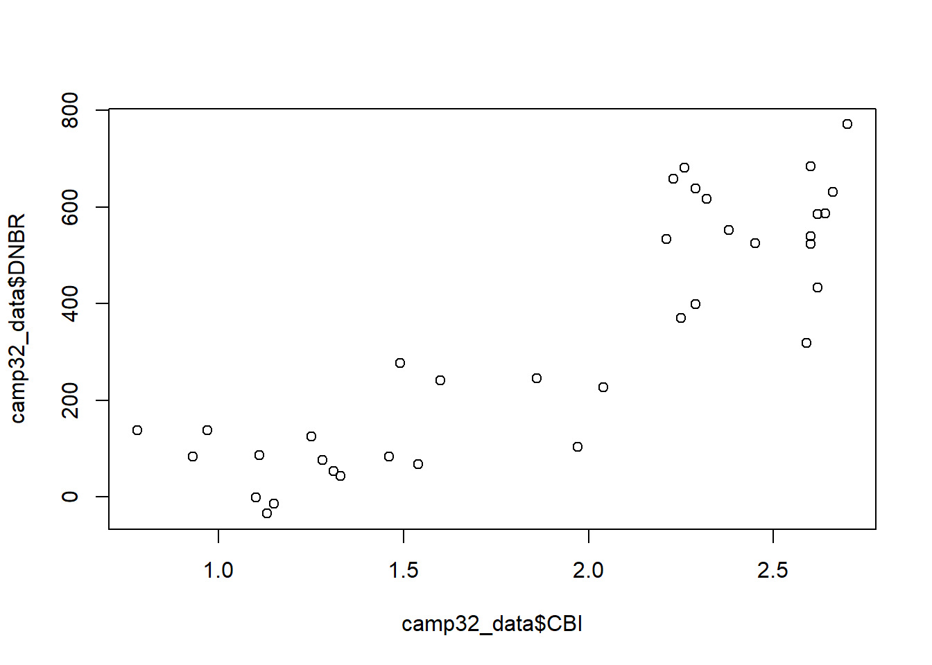
When a plotting function is run, its output is sent to a graphical device. If you are working in RStudio, the build-in graphical device is located in the lower right-hand pane in the Plots tab. The plot can be copied or saved to a graphics file using the Export button, and it can be expanded using the Zoom button.
To make a neater looking plot, a title and axis labels can be specified as additional arguments to the plot() function.
plot(x=camp32_data$CBI, y=camp32_data$DNBR,
     main = "Camp 32 Fire Severity",
     xlab="CBI",
     ylab="DNBR")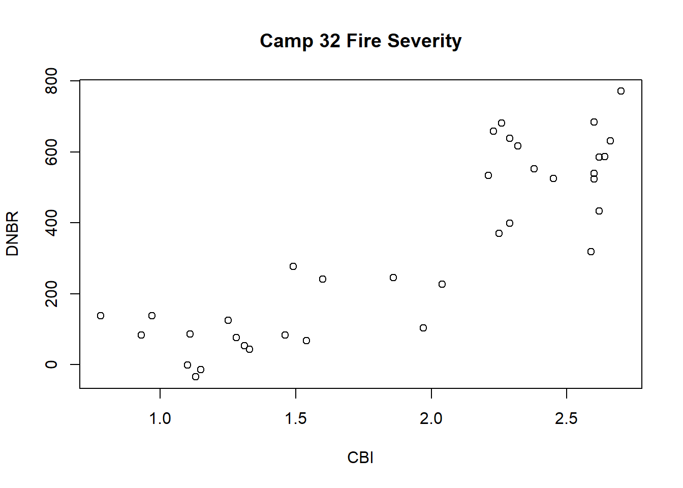
The hist() function is used here to generate a histogram of the DNBR values. Because a histogram is a univariate plot, only a single vector of data is provided as the x argument along with a title and x-axis label.
hist(x=camp32_data$DNBR,
     main = "Differenced Normalized Burn Ratio",
     xlab = "DNBR")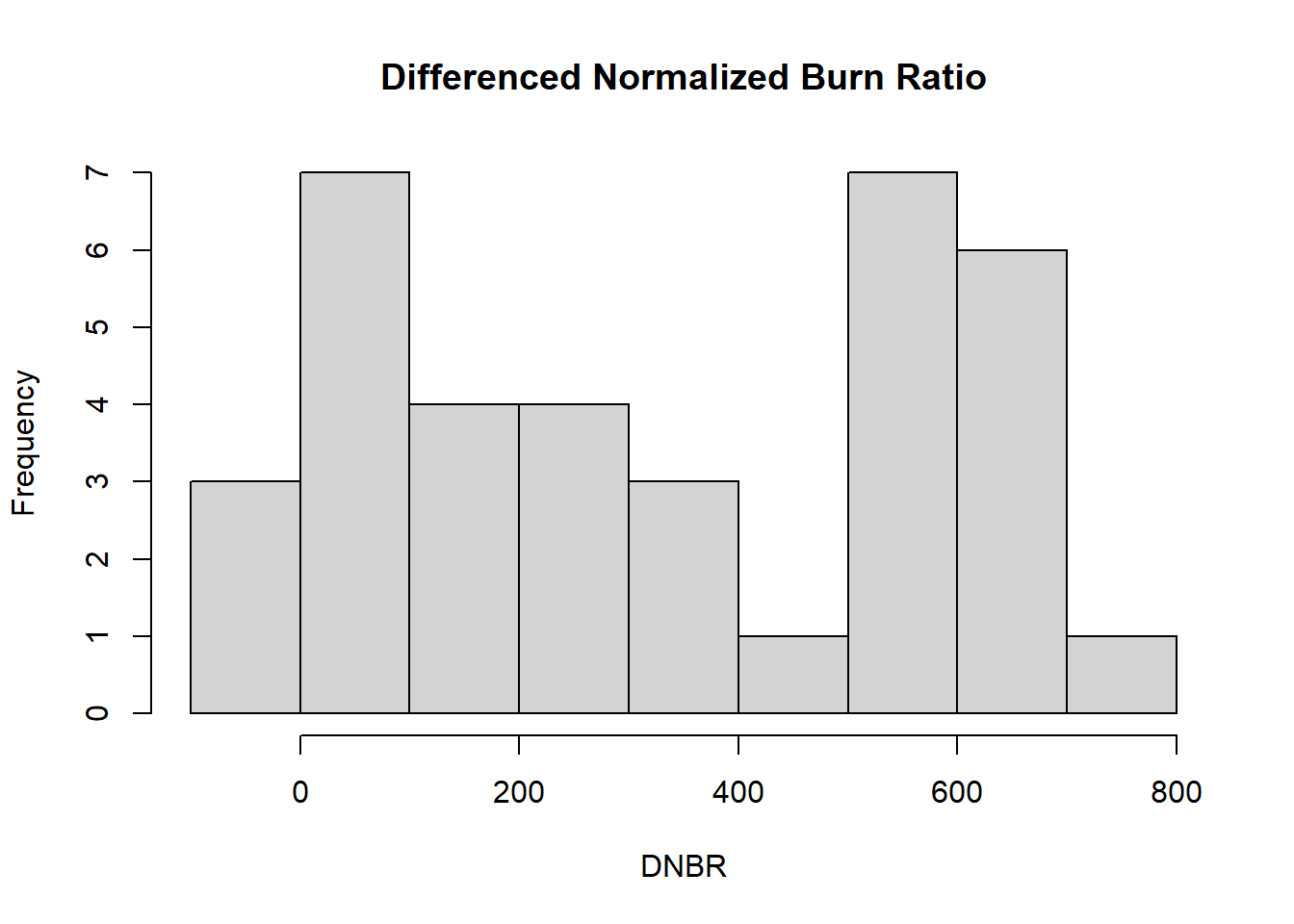
To compare the distributions of fire severity in plots with different types of fuel treatments, the boxplot() function can be used. The arguments for this type of plot are different from the preceding examples. The first argument is a formula, DNBR ~ PLOT_CODE, which can be interpreted as “DNBR as a function of PLOT_CODE.” The data argument specifies the data frame containing these columns, and additional arguments provide a title and axis labels.
boxplot(DNBR ~ PLOT_CODE, data = camp32_data,
        main = "Treatment Effects on Fire Severity",
        xlab="Treatment Type",
        ylab="DNBR")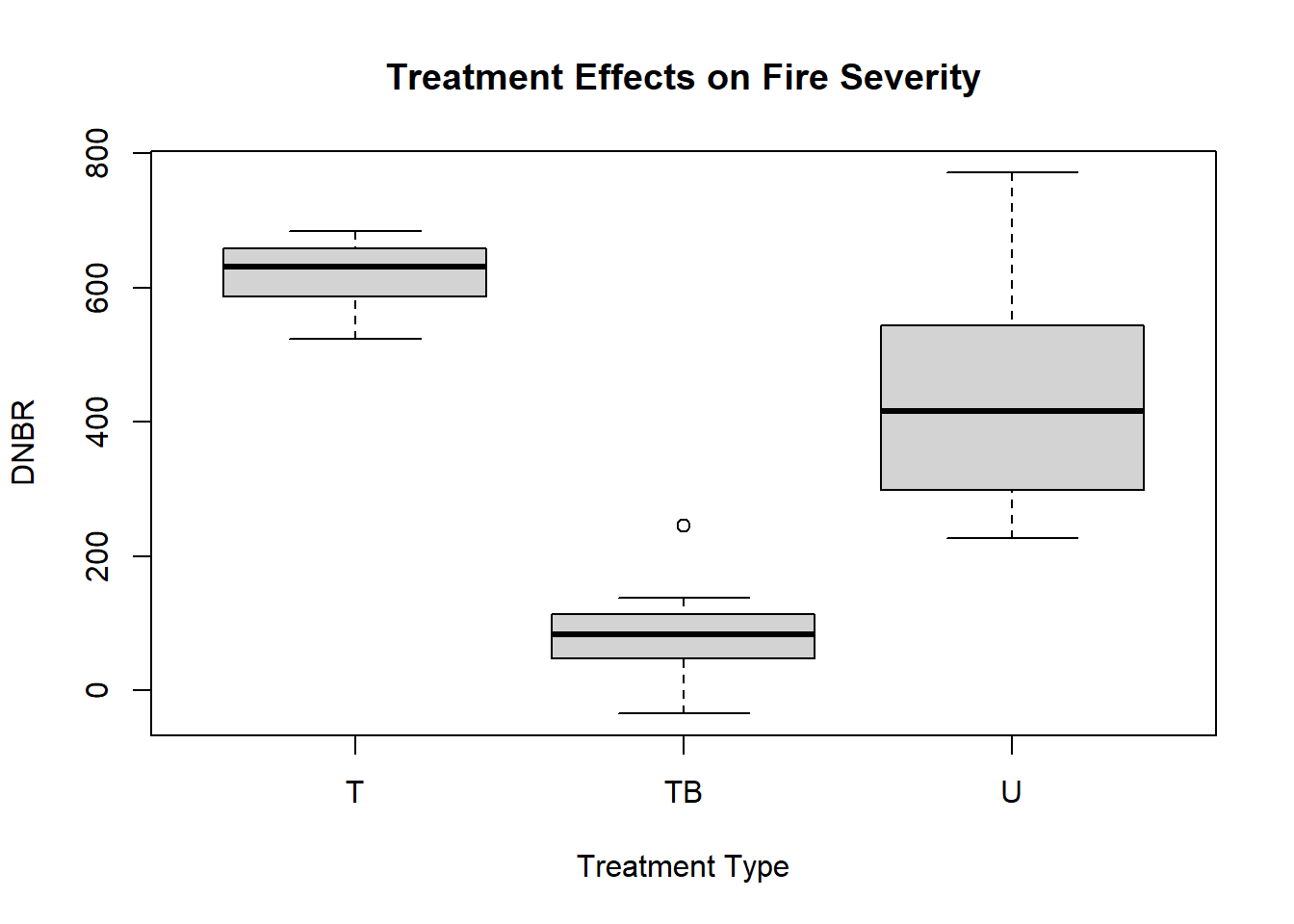
Knowing the arguments that can be specified for a specific function is very important. The quickest way to learn more about an R function is to display its documentation using the help() function. This function provides access to manual pages with information about function arguments, details about what the function does, and a description of the output that is produced. In RStudio, the help pages are displayed in the Help tab in the lower right hand window.
help(plot)1.3.2 Statistical analysis
Functions are also used to carry various types of statistical tests in R. For example, the t.test() function can be used to compute confidence intervals for the mean of a variable. The x argument is the vector of data. The conf.level argument specifies the probability of the confidence intervals. Note that if no conf.level argument is provided, a 95% confidence interval is produced.
t.test(x=camp32_data$DNBR)##
## One Sample t-test
##
## data: camp32_data$DNBR
## t = 7.963, df = 35, p-value = 2.286e-09
## alternative hypothesis: true mean is not equal to 0
## 95 percent confidence interval:
## 248.2493 418.1396
## sample estimates:
## mean of x
## 333.1944t.test(x=camp32_data$DNBR, conf.level=0.9)##
## One Sample t-test
##
## data: camp32_data$DNBR
## t = 7.963, df = 35, p-value = 2.286e-09
## alternative hypothesis: true mean is not equal to 0
## 90 percent confidence interval:
## 262.4982 403.8907
## sample estimates:
## mean of x
## 333.1944t.test(x=camp32_data$DNBR, conf.level=0.99)##
## One Sample t-test
##
## data: camp32_data$DNBR
## t = 7.963, df = 35, p-value = 2.286e-09
## alternative hypothesis: true mean is not equal to 0
## 99 percent confidence interval:
## 219.2231 447.1658
## sample estimates:
## mean of x
## 333.1944How does the t.test() function know what confidence level to use if we do not specify the conf.level argument? In many cases, arguments have a default value. If the argument is not specified in the function call, then the default value is used. When using statistical fundtions in R, it is particularly important to study the documentation to learn the default values and decide if they are appropriate for the analysis.
help(t.test)To conduct a two-sample t-test, the same function is used with two arguments, x and y, which are the two sets of data to be compared. In the code below, two new vectors are created from the camp32_data data frame. U_DNBR contains DNBR values from the untreated plots and TB_DNBR contains DNBR values from the thinned and burned plots.
U_DNBR <- camp32_data[camp32_data$PLOT_CODE == "U", "DNBR"]
TB_DNBR <- camp32_data[camp32_data$PLOT_CODE == "TB", "DNBR"]
t.test(x=U_DNBR, y=TB_DNBR)
##
## Welch Two Sample t-test
##
## data: U_DNBR and TB_DNBR
## t = 7.0902, df = 14.174, p-value = 5.058e-06
## alternative hypothesis: true difference in means is not equal to 0
## 95 percent confidence interval:
## 248.8065 464.2602
## sample estimates:
## mean of x mean of y
## 436.3333 79.8000The next example is a linear regression of the field-based burn severity index (CBI) as a function of the satellite-derived burn severity index (DNBR). The lm() function takes two arguments, a formula and a data argument, and returns an object belonging to class lm. Note that the lm object is really just a list object whose elements contain various pieces of information about the regression results.
camp32_lm <- lm(CBI ~ DNBR, data=camp32_data)
class(camp32_lm)
## [1] "lm"attributes(camp32_lm)## $names
## [1] "coefficients" "residuals" "effects" "rank"
## [5] "fitted.values" "assign" "qr" "df.residual"
## [9] "xlevels" "call" "terms" "model"
##
## $class
## [1] "lm"To obtain more interpretable results, we can then use various other functions to summarize the lm object and to extract coefficients, fitted values, and residuals. These results are used to generate a residual plot and check to see if linear regression assumptions such as linearity and homoskedasticity are met.
# Summary of basic regression results
summary(camp32_lm)
##
## Call:
## lm(formula = CBI ~ DNBR, data = camp32_data)
##
## Residuals:
## Min 1Q Median 3Q Max
## -0.69976 -0.20237 0.00781 0.18838 0.71515
##
## Coefficients:
## Estimate Std. Error t value Pr(>|t|)
## (Intercept) 1.1785297 0.0867154 13.59 2.66e-15 ***
## DNBR 0.0021828 0.0002089 10.45 3.75e-12 ***
## ---
## Signif. codes: 0 '***' 0.001 '**' 0.01 '*' 0.05 '.' 0.1 ' ' 1
##
## Residual standard error: 0.3103 on 34 degrees of freedom
## Multiple R-squared: 0.7625, Adjusted R-squared: 0.7555
## F-statistic: 109.2 on 1 and 34 DF, p-value: 3.746e-12# Regression coefficients
coef(camp32_lm)## (Intercept) DNBR
## 1.17852968 0.00218282# Residuals
resid(camp32_lm)## 1 2 3 4 5
## -0.6997589065 -0.4318866017 -0.5097589065 -0.0763468627 -0.2562522426
## 6 7 8 9 10
## 0.0256862125 -0.0001530172 -0.2013822405 -0.0644240380 0.0157808325
## 11 12 13 14 15
## 0.0554262167 0.0981133983 -0.2931709503 0.2130385256 -0.1067722342
## 16 17 18 19 20
## 0.1466793044 0.5644569891 0.3659700726 -0.1341558083 -0.3848255452
## 21 22 23 24 25
## 0.2638267470 -0.4072132363 -0.2833519565 0.2405249537 -0.2053299064
## 26 27 28 29 30
## -0.0056293970 0.1254895758 0.7151505904 0.2427472689 0.2776723963
## 31 32 33 34 35
## -0.0715788772 0.1645203483 0.4941262376 0.1801547074 0.1041106072
## 36
## -0.1614842571# Fitted values
fitted(camp32_lm)## 1 2 3 4 5 6 7 8
## 1.479759 1.361887 1.479759 1.176347 1.366252 1.104314 1.150153 1.451382
## 9 10 11 12 13 14 15 16
## 1.344424 1.294219 1.274574 1.361887 1.783171 1.326961 1.706772 1.713321
## 17 18 19 20 21 22 23 24
## 1.405543 1.674030 2.344156 2.614826 1.986173 2.667213 2.573352 2.049475
## 25 26 27 28 29 30 31 32
## 2.525330 2.385629 2.324510 1.874849 2.357253 2.322328 2.671579 2.455480
## 33 34 35 36
## 2.125874 2.459845 2.555889 2.861484plot(x=fitted(camp32_lm), y=resid(camp32_lm))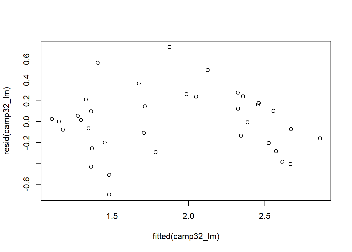
-
From the Camp 32 dataset, extract a vector containing the CBI values from the untreated plots (treatment code U) and another containing the CBI values for the thinned/unburned plots (treatemnt code T). Conduct a two-sample t-test comparing the mean CBI for these two treatment types.
-
Generate a histogram plot of CBI values and compare it with the histogram of DNBR values.
-
Generate a new version of the DNBR versus CBI scatterplot with an aspect ratio of 1 (equal length of x and y axes). To do this, you will need to specify an additional argument. Consult the help page for the base
plot()function to find the name of the argument to use.