10 A text project, from start to topic model
In this tutorial, we focus on a new analysis strategy for text - topic modeling. We download all of the pages on Wikipedia for famous philosophers, from Aristotle to Bruno Latour. Each page discusses their lives and works and we topic model the text in order to identify shared themes across them.
To do this, we first need to load in a bunch of packages. If you are missing one of these packages - if you get the error message “Error in library(tm) : there is no package called ‘tm’”, for example - then you should use install.packages() to install it.
In particular, there are three packages we have never seen before: stringi, which is useful for manipulating strings (we will use it to convert non-latin script to latin script), tm, which is a suite of functions for text mining in R, and texclean, which has useful functions for cleaning text.
library(rvest)
library(tidytext)
library(dplyr)
library(tidyr)
library(stringi)
library(tm)
library(textclean)
Most of the real scraping work I left out of the tutorial for the sake of time. But I followed, more or less, what we learned in the week on scraping. I found a page a series of pages which list philosophers alphabetically. I visited those pages and saw that they contained links to every Wikipedia page for a well-known philosopher. I used Inspect to copy the Xpath for a couple of these links and found that they followed a similar pattern - each was nested in the HTML structure underneath the pathway //*[@id=“mw-content-text”]/div/ul/li/a. I extracted the set of nodes which followed that path and grabbed the href (HTML lingo for a url) from each. The result was a list of Wikipedia short links for philosophers. I pasted the main wikipedia URL to precede short links. I also grabbed the titles of the nodes, which was the names of the philosophers. I used lapply to apply this function to each of the four pages, saved the results for each in a data.frame, and used do.call(“rbind”) to put all of them into a single data.frame.
grab_urls <- function(x){

  # id the url locations on the page (identified using Inspect and XPath)
  philosophers_urls <- html_nodes(x, xpath = '//*[@id="mw-content-text"]/div/ul/li/a')

  # extract the URL specifically
  href_links <- philosophers_urls %>% html_attr('href')

  # paste the url ending to wikipedia English main url
  urls <- paste0("https://en.wikipedia.org/", href_links)

  # extract each philosopher's name
  philosopher_names <- philosophers_urls %>% html_attr('title')

  # save the result in a data.frame
  df <- data.frame(Philosopher = philosopher_names, URL = urls, stringsAsFactors = F)

  # output the data.frame
  return(df)
}

# download html for each of the main philosopher pages from wikipedia
philosophers_A_C <-  read_html("https://en.wikipedia.org/wiki/List_of_philosophers_(A–C)")
philosophers_D_H <- read_html("https://en.wikipedia.org/wiki/List_of_philosophers_(D–H)")
philosophers_I_Q <- read_html("https://en.wikipedia.org/wiki/List_of_philosophers_(I–Q)")
philosophers_R_Z <- read_html("https://en.wikipedia.org/wiki/List_of_philosophers_(R–Z)")

# apply the above code to each of the pages
all_dfs <- lapply(list(philosophers_A_C, philosophers_D_H, philosophers_I_Q, philosophers_R_Z), grab_urls)

# put it all together
all_philosophers <- do.call("rbind", all_dfs)
Let’s take a look. The data.frame has two columns - Philosopher and URL. We can use this information to now go to each of the philosopher’s pages and grab the content of their Wikipedia page.
So now I write a new function which grabs the text from each page. It takes as its argument a URL. The HTML of this URL is read into R using rvest’s read_html. Then the body of the page - identified by //*[@id=“mw-content-text”]/div/p - is read into R and its text is extracted. This text is returned.
grab_text <- function(x){
    philosopher_html <- read_html(x)
    philosopher_text <- philosopher_html %>%
      html_nodes(xpath = '//*[@id="mw-content-text"]/div/p') %>%
      html_text()
  return(philosopher_text)
}
I apply it, again using lapply, to every URL in the all_philosophers data.frame. The result is the text of every philosopher’s page on Wikipedia. The only problem is it takes a while to run, especially if your computer isn’t fast.
I actually saved the results into an RDS file and put them on Canvas, so that you wouldn’t have to run this full loop (though you can if you are curious.) Download philosophers_page_text.RDS, drag it into your R directory, and load it in using readRDS, like so.
So the texts are quite messy and we need to clean them before we can analyze them (though with topic modeling, this isn’t strictly necessary since it will often lump all of the junk into its own topic.) We build a function to do that. It uses repeated gsubs to remove characters that we don’t want from the text. If you don’t really understand what is going on here, then it is worth reading up on regex - it is an essential framework for working with text. Once the text is cleaned, we put all of the sentences for each philosopher into a single character vector and make it lowercase. Finally, we convert the list of texts to a character vector
clean_text <- function(x){
  # remove all parentheses and their content
  x <- gsub("\\s*\\([^\\)]+\\)", "", x)
  # remove all square brackets and their content
  x <- gsub("\\[[^][]*]", "", x)
  # remove all punctuation
  x <- gsub('[[:punct:] ]+',' ',x)
  # remove all numbers
  x <- gsub('[[:digit:]]+', '', x)
  # drop paragraph breaks
  x <- gsub('\n', '', x)
  # drop empty lines
  x <- subset(x, x != "")
  # remove spaces at beginning and end of lines
  x <- trimws(x)
  # paste all of the lines together into one text
  x <- paste0(x, collapse = " ")
  # make everything lower case
  x <- tolower(x)
  # return text
  return(x)
}

philosophers_texts_cleaned <- unlist(lapply(philosophers_page_text, clean_text))
Now we can add the texts into the data.frame of philosophers and their URLs. We can also drop the philosophers whose name was on Wikipedia but who don’t actually have a page. They can be identified by the fact that their text equals “error in open connection http error”.
# convert non-latin script to latin, if no easy conversion, then substite for empty string (i.e. delete)
philosophers_texts_cleaned <- iconv(stri_trans_general(philosophers_texts_cleaned, "latin-ascii"), "latin1", "ASCII", sub="")
philosophers_texts_cleaned <- replace_non_ascii(philosophers_texts_cleaned)
good_texts <- which(philosophers_texts_cleaned!= "error in open connection http error")

all_philosophers <- all_philosophers[good_texts,]
all_philosophers$Text <- philosophers_texts_cleaned[good_texts]
Now we have to do some more cleaning. We can turn this data set into a tokenized tidytext data set with the unnest_tokens function.
# further cleaning...
# tokenize the result
text_cleaning_tokens <- all_philosophers %>% unnest_tokens(word, Text)
Next we want to drop words which are less than three characters in length, and drop stop words. We can drop short words with filter combined with the nchar function, and anti_join to drop stopwords.
# drop words with are either stop words or length == 1
text_cleaning_tokens <- text_cleaning_tokens %>%
  filter(!(nchar(word) < 3)) %>%
  anti_join(stop_words)
## Joining, by = "word"Next we drop empty words
The next part is a bit complicated. The basic idea is that we want to paste the texts for each philosopher back together. The unite function is good for that, but it only works on a wide form data set. So we will first group by philosopher, produce an index for the row number (that is, what position is a given word in their text), we will then spread the data, converting our long form data into wide form, setting the key argument (which defines the columns of the new data.frame) to equal the index we created, and the value argument to word. The result is that each book is now its own row in the data.frame, with the column i+2 identifying the ith word in that philosopher’s Wikipedia page.
# turn each person into a row, with a column for each word in their wikipedia
tokens <- tokens %>% group_by(Philosopher) %>%
  mutate(ind = row_number()) %>%
  spread(key = ind, value = word)
We’ll convert NAs to "" and use unite to paste all of the columns in the data.frame together. We specify -Philosopher and -URL so that those columns are preserved and not pasted with the words of each page.
# convert NAs to empty strings
tokens[is.na(tokens)] <- ""

# put the data.frame back together
tokens <- unite(tokens, Text,-Philosopher, -URL, sep =" " )
Two last things are necessary before we analyze the data. We need to trim whitespace, so that there aren’t spaces at the beginning or end of texts. And we need to convert non-latin characters to latin characters (using the stri_trans_general() function from stringi) or else, if they can’t be converted, drop them (using the iconv() function from base R.)
Great! Let’s check out the data.
Topic modeling requires a document to word matrix. In such a matrix, each row is a document, each column is a word, and each cell or value in the matrix is a count of how many times a given document uses a given word. To get to such a matrix, we first need to count how many times each word appears on each philosopher’s page. We learned how to do this last tutorial.
Now we can use a function called cast_dtm from the tm package to convert token_counts into a document-to-word matrix (dtm stands for document-to-term, actually.) We tell it - the variable in token_counts we want to use for the rows of the dtm (Philosopher), the variable we want to use as the column (word), and the variable that should fill the matrix as values (n).
Awesome! You can View what it looks like if you want. We can use this dtm to fit a topic model using latent dirichlet allocation (LDA) from the topicmodels package. We have a few options when doing so - first we will set k, the number of topics to equal 20. If we were doing this for a real study (like your final project), we would want to fit a couple of different models with different ks to see how the results change and to try to find the model with the best fit. For now, we will settle for just trying k = 20. We can also set the seed directly inside the function so that we are certain to all get the same results.
This might take a while!
## Warning: package 'topicmodels' was built under R version 3.6.2##
## Attaching package: 'topicmodels'## The following object is masked from 'package:text2vec':
##
## perplexityIt finished running - now what? We can use the tidy function from the tidyr package to extract some useful information. First, let’s extract the beta coefficients - which provides weights for the words with respect to topics.
Just like we did last class, let’s use top_n to grab the top 10 words per topic.
top_terms <- philosophers_lda_td %>%
  group_by(topic) %>%
  top_n(10, beta) %>%
  ungroup() %>%
  arrange(topic, -beta)
We can plot the results using ggplot as a series of bar plots
library(ggplot2)

top_terms %>%
  mutate(term = reorder_within(term, beta, topic)) %>%
  ggplot(aes(term, beta)) +
  geom_bar(stat = "identity") +
  scale_x_reordered() +
  facet_wrap(~ topic, scales = "free_x") +
  theme_bw()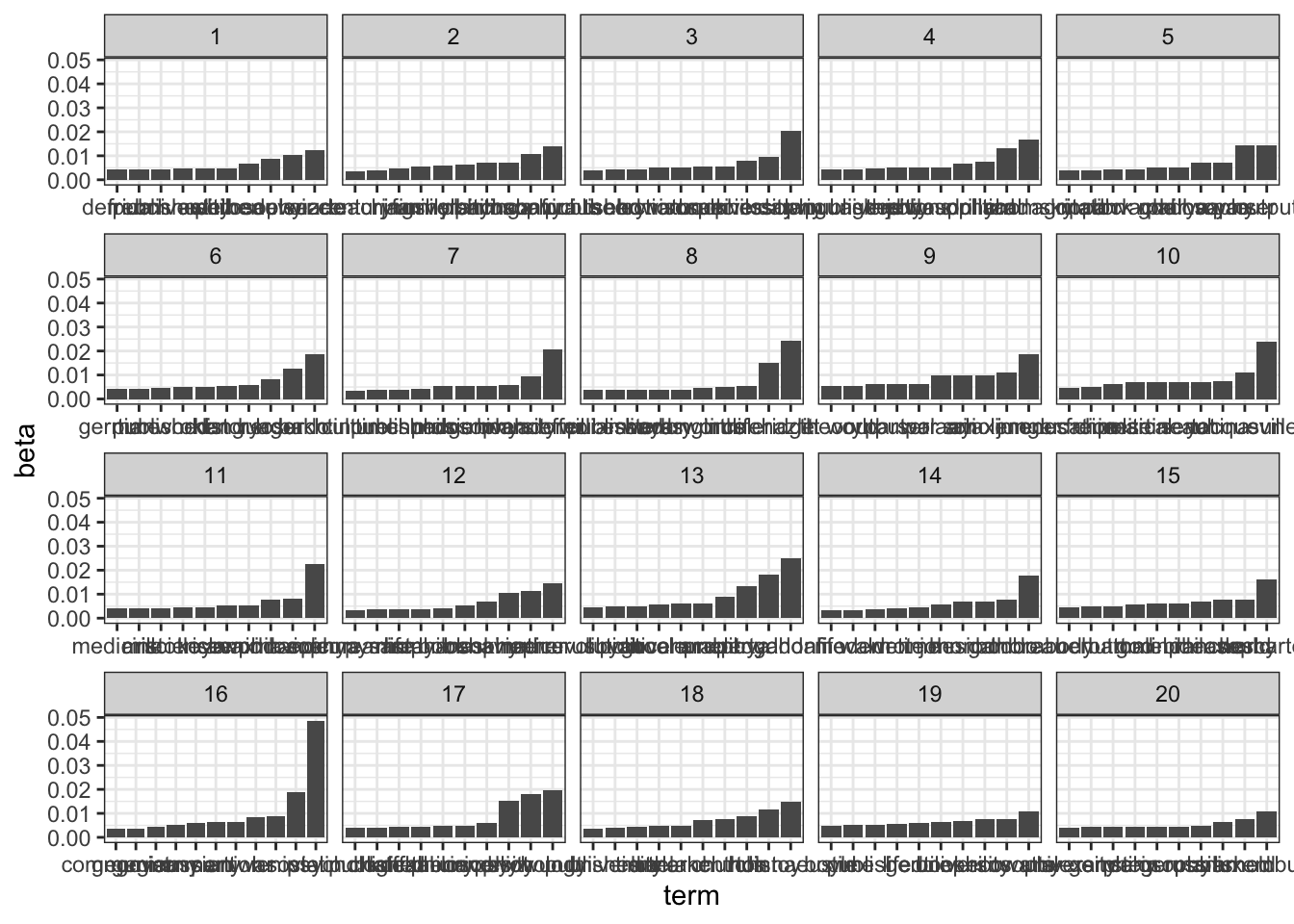
Or else as a table.
top_terms_table <- top_terms %>%
  group_by(topic) %>%
  mutate(order = 1:length(topic)) %>%
  select(-beta) %>%
  spread(topic, term) %>%
select(-order) | 1 | 2 | 3 | 4 | 5 | 6 | 7 | 8 | 9 | 10 | 11 | 12 | 13 | 14 | 15 | 16 | 17 | 18 | 19 | 20 |
|---|---|---|---|---|---|---|---|---|---|---|---|---|---|---|---|---|---|---|---|
| psychology | philosophy | wittgenstein | law | plato | king | political | french | university | ibn | german | church | mao | parser | philosophy | chamberlain | john | god | darwin | law |
| university | french | philosophy | guevara | life | burke | party | rousseau | philosophy | jewish | published | god | chinese | output | theory | eliade | smith | church | reich | buddha |
| priestley | heidegger | shankara | bacon | greek | hume | government | voltaire | professor | god | philosophy | john | gandhi | socrates | logic | time | published | christian | time | foucault |
| peirce | freud | russell | hayek | aristotle | kafka | stalin | published | college | islamic | hegel | pope | china | background | social | leibniz | church | origen | wallace | kant |
| wundt | world | gibbs | published | diogenes | steiner | marx | paris | theory | philosophy | time | thomas | sun | lock | science | newton | william | life | adorno | theory |
| arendt | university | school | linnaeus | philosophy | schopenhauer | war | time | philosopher | arabic | friedrich | aristotle | people | gray | world | galileo | wrote | gregory | published | legal |
| philosophy | published | time | time | time | world | soviet | france | oxford | time | goethe | luther | government | fondane | mind | gobineau | time | kierkegaard | wrote | buddhist |
| published | derrida | university | university | world | published | revolution | wrote | published | taymiyyah | wrote | theology | political | turing | knowledge | wrote | college | theology | evolution | kelsen |
| chomsky | husserl | god | erasmus | blake | time | lenin | book | school | wrote | germany | time | life | citation | university | kepler | england | augustine | huxley | jung |
| research | theory | life | wrote | pythagoras | life | social | diderot | science | maimonides | life | century | han | published | human | descartes | english | christ | natural | time |
What if want to look at the extent to which each document or philosopher is composed of each topic? We can instead set matrix = “gamma” to get the gamma values, which tell you exactly that.
We’ll sort in descending order according to gamma
There are a bunch of philosophers, too many to examine all at once. Let’s select a few particularly prominent ones and examine their topic distributions.
selected_philosophers <- c("Martin Luther King, Jr.",
  "Francis Bacon",
  "Wang Fuzhi",
  "Aristotle",
  "Immanuel Kant",
  "Pope John XXI",
  "Friedrich Kayek",
  "Edmund Burke",
  "Simone de Beauvoir",
  "Bruno Latour")

top_topics %>%
  filter(document %in% selected_philosophers) %>%
  ggplot(aes(topic, gamma)) +
  geom_bar(stat = "identity") +
  scale_x_continuous(breaks=1:20) +
  facet_wrap(~ document, scales = "free") +
  theme_bw()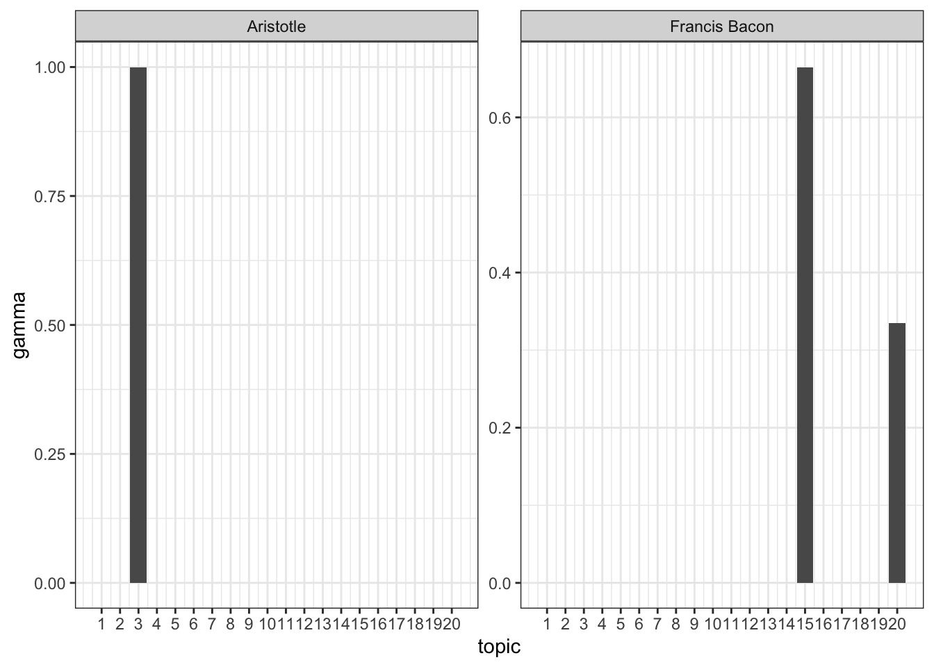
10.0.1 LAB
For the lab this week, select or randomly sample 100 texts from the Gutenberg library and topic model the texts with a k of your choosing.