A Solutions to Exercises

A.1 Section 3 Data Structures

A.1.1 3.4 Data frames

A.1.1.0.1 Exercise 1: What is the difference between cbind and rbind? C = columns, R = rows

bind() and rbind() both create matrices or data frames by combining several vectors of the same length. cbind() combines vectors as columns, while rbind() combines them as rows.

A.1.1.0.2 Exercise 2: We found out that the blood pressure instrument is under-recording each measure and all measurement incorrect by 0.1. How would you add 0.1 to all values in the blood vector?**

id     <- c("N198","N805","N333","N117","N195","N298")
gender <- c(1, 0, 1, 1, 0, 1)  # 0 denotes male, 1 denotes female
age    <- c(30, 60, 26, 75, 19, 60)
blood  <- c(0.4, 0.2, 0.6, 0.2, 0.8, 0.1)

my_data <- data.frame(id, gender, age, blood)
my_data <- data.frame(ID = id, Sex = gender, Age = age, Blood = blood)
my_data

##     ID Sex Age Blood
## 1 N198   1  30   0.4
## 2 N805   0  60   0.2
## 3 N333   1  26   0.6
## 4 N117   1  75   0.2
## 5 N195   0  19   0.8
## 6 N298   1  60   0.1

blood #here we see the original blood measures before we apply any changes

## [1] 0.4 0.2 0.6 0.2 0.8 0.1

updated_blood <- (blood) + 0.1 #we have added 0.1 to all values in the blood vector
updated_blood #we check if the changes have been applied

## [1] 0.5 0.3 0.7 0.3 0.9 0.2

A.1.1.1 Exercise 3: We found out that the first patient is 33 years old. How would you change the first element of the vector age to 33 years?

my_data #here we see that the first patient age is 30yo

##     ID Sex Age Blood
## 1 N198   1  30   0.4
## 2 N805   0  60   0.2
## 3 N333   1  26   0.6
## 4 N117   1  75   0.2
## 5 N195   0  19   0.8
## 6 N298   1  60   0.1

my_data[1, "Age"] <- 33 #we changed it to 33yo
my_data$Age #we check if the changes have been applied

## [1] 33 60 26 75 19 60

A.2 Section 4 Handling data: the Tidyverse

iris

A.2.0.0.1 Exercise 1. Select only the columns Sepal.Length and Sepal.Width

select(iris, Sepal.Length, Sepal.Width)

#equivalent to
iris[, c(1,2)]

A.2.0.1 Exercise 2. Arrange the data by increasing Sepal.Length

arrange(iris, (Sepal.Length))

A.2.0.2 Exercise 3. Filter the data to only include Species setosa.

filter(iris, Species == "setosa")

A.2.0.3 Exercise 4. Select the columns Petal.Length and Petal.Width, then make (mutate) a new column Petal.Area as Petal.Length multiplied by Petal.Width, then arrange in order of decreasing petal area.

Petal.Area <- mutate(iris,
       Petal.Area = Petal.Length * Petal.Width)

arrange(iris, desc(Petal.Area))

4.2 More dplyr verbs: group_by and summarise

A.2.0.4 Exercise 1. group_by species and calculate the mean Petal.Length for each species.

iris_by_species <- group_by(iris, Species)
iris_by_species

A.2.0.5 Exercise 2. group_by species, then standardise the Petal.Length within each species – i.e. subtract the mean and divide by the standard deviation. Hint: your processed dataset should still have 150 rows; you will need to use mutate rather than

A.3 Section 5: Getting data in and out of R

Set a working directory by: 1. setwd or 2. Session > Set Working Directory

read.csv("CHD2019.csv")

A.4 Section 6: Control Structures: loops and conditions

A.4.0.1 6.1. if, else and for

Fizz Buzz exercise

The most obvious way of solving FizzBuzz is to loop through a set of integers. In this loop, we use conditional statements to check whether each integer is divisible by 3 and/or 5.

for (i in 1:100){
  if(i %% 15 == 0){
    print("fizz-buzz")
  } else if(i %% 3 == 0){
    print("fizz")
  } else if(i %% 5 == 0){
    print("buzz")
  } else {
    print(i)
  }
}

A.5 Section 7 Writing your own functions

fizz_buzz <- function(n){
  x <- 1:n
  y <- x
  y[x %% 3 == 0] <- "fizz"
  y[x %% 5 == 0] <- "buzz"
  y[x %% 15 == 0] <- "fizz-buzz"
  y
}

fizz_buzz(100)

##   [1] "1"         "2"         "fizz"      "4"         "buzz"      "fizz"      "7"         "8"         "fizz"      "buzz"      "11"       
##  [12] "fizz"      "13"        "14"        "fizz-buzz" "16"        "17"        "fizz"      "19"        "buzz"      "fizz"      "22"       
##  [23] "23"        "fizz"      "buzz"      "26"        "fizz"      "28"        "29"        "fizz-buzz" "31"        "32"        "fizz"     
##  [34] "34"        "buzz"      "fizz"      "37"        "38"        "fizz"      "buzz"      "41"        "fizz"      "43"        "44"       
##  [45] "fizz-buzz" "46"        "47"        "fizz"      "49"        "buzz"      "fizz"      "52"        "53"        "fizz"      "buzz"     
##  [56] "56"        "fizz"      "58"        "59"        "fizz-buzz" "61"        "62"        "fizz"      "64"        "buzz"      "fizz"     
##  [67] "67"        "68"        "fizz"      "buzz"      "71"        "fizz"      "73"        "74"        "fizz-buzz" "76"        "77"       
##  [78] "fizz"      "79"        "buzz"      "fizz"      "82"        "83"        "fizz"      "buzz"      "86"        "fizz"      "88"       
##  [89] "89"        "fizz-buzz" "91"        "92"        "fizz"      "94"        "buzz"      "fizz"      "97"        "98"        "fizz"     
## [100] "buzz"

A.6 Section 9: Introduction to plotting

swiss

plot(density(swiss$Fertility),type="1")

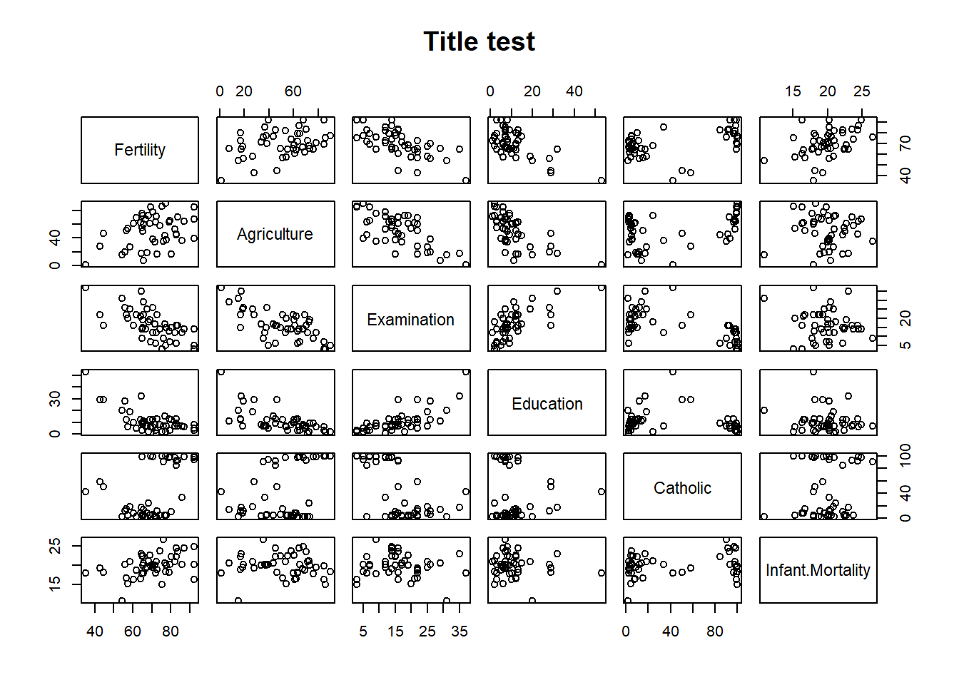
Exercise: Take a look at all different values that can be used for type using the help manual

?type

Exercise: Choose another data set and recreate these plots for variables of your choice

Try data() to get a list of built-in data sets and their dependency packages. Then use the code provided in the Intro to R course to recreate the plots with a dataset of your choice. !NB there are several ways that these plots can be recreated. :-)

data() 

Exercise: Try and work out how to change the title of the plot.

plot(swiss, main = "Title test")