10Confounding and Interaction in Logistic Regression
Learning objectives
By the end of this week you should be able to:
Interpret statistical output for a multiple logistic regression model with interactions
Understand how predicted values and residuals can be extended to this model
Learn about prediction and residuals in this setting
Discover how to identify outliers and influential observations
Understand how to use these tools to assess the model fit
Learning activities
This week’s learning activities include:
Learning Activity
Learning objectives
Lecture 1
1, 2, 3
Reading
1,
Lecture 2
2, 3, 4, 5
Practice/Investigation
1, 3
Discussion
all
Lecture 1 in R
Lecture 1 in Stata
Interactions
The interaction between two X variables, also known as effect modification, in logistic regression is similar to what we saw in linear regression. With logistic regression, the interpretation is typically done in terms of OR (whereas the interaction term is typically added on the log-odds scale). This deserves explanation. The general form of an interaction model with two covariates \(x_1\) and \(x_2\) is: \(logit(p)= \beta_0 + \beta_1 x_1 + \beta_2 x_2 + \beta_3 x_1\times x_2\) where \(logit(p)\) is shortened version of \(\log(p/(1-p))\) and, for simplicity, we have simplified the notation since \(p=p(y=1 | x_1, x_2, x_1\times x_2)\). Also \(x_1\) and \(x_2\) can be binary or continuous with the convention that a binary indicator is always coded 0/1.
Interaction between two binary variables
We again consider the WCGS study and consider the potential interaction between arcus and a binary indicator for patients aged over 50 called bage_50. The specification of the logistic model in Stata or R follows the general syntax used with the linear model. You can either define “by hand” the interaction term and add it to the model with the the two covariates arcus and bage_50 or let the software do the job for you. We will use the second approach here and note that it is critical to use the coding (0/1) or to tell Stata or R to create the right indicators for you. The Stata syntax will then be: logistic chd69 i.arcus##i.bage_50, coef and R’s: glm(chd69\(\sim\) factor(arcus)\(*\)factor(bage_50), family=binomial, data=wcgs). The command factor() is not necessary when both covariates are coded 0/1. Note that in the Stata command we used the option coef to avoid reporting the ORs. The following results are obtained:
R code and output
Show the code
wcgs <-read.csv("wcgs.csv")wcgs<-data.frame(wcgs)wcgs$bage_50<-as.numeric(wcgs$age>=50)out1<-glm(chd69 ~ arcus*bage_50, family=binomial, data=wcgs)summary(out1) ## ## Call:## glm(formula = chd69 ~ arcus * bage_50, family = binomial, data = wcgs)## ## Coefficients:## Estimate Std. Error z value Pr(>|z|) ## (Intercept) -2.8829 0.1089 -26.467 < 2e-16 ***## arcus 0.6480 0.1789 3.623 0.000292 ***## bage_50 0.8933 0.1721 5.190 2.11e-07 ***## arcus:bage_50 -0.5921 0.2722 -2.175 0.029640 * ## ---## Signif. codes: 0 '***' 0.001 '**' 0.01 '*' 0.05 '.' 0.1 ' ' 1## ## (Dispersion parameter for binomial family taken to be 1)## ## Null deviance: 1771.2 on 3151 degrees of freedom## Residual deviance: 1730.9 on 3148 degrees of freedom## (2 observations deleted due to missingness)## AIC: 1738.9## ## Number of Fisher Scoring iterations: 5
The interaction term is significant (\(p=0.03\)) which means that we cannot ignore the age effect when considering the association of arcus with CHD. Let’s use the notation introduced above, \(x_1\) = arcus and \(x_2\) = bage_50 and consider a young patient (less than 50) without arcus. The log-odds of CHD occurrence is: \(\hat\beta_0=-2.88\) up to rounding. Compare with someone in the same age category with arcus, the log-odds of CHD occurrence is: \(\hat\beta_0+\hat\beta_1=-2.23\), therefore the OR for arcus in this age group is: \(\exp(\hat\beta_0+\hat\beta_1)/\exp(\hat\beta_0)=\exp(\hat\beta_1)=1.91\), 95\(\%\)CI=(1.34 ; 2.70). By the same token, the log-odds of CHD occurence for a patient aged 50+ without arcus is: \(\hat\beta_0+\hat\beta_2=-2.88+.89=-1.99\) and changes to \(\hat\beta_0+\hat\beta_1+\hat\beta_2+\hat\beta_3=-1.93\) for patients with arcus, therefore the OR for arcus in patients aged 50+ is \(\exp(\hat\beta_1+\hat\beta_3)=1.06\) by taking the ratio of the corresponding exponentiated terms. To get a 95\(\%\) CI for this OR we need to use lincom or the corresponding R command yielding OR=1.06, 95\(\%\)CI=(0.71 ; 1.58).
R code and output
Show the code
library(multcomp)## Loading required package: mvtnorm## Loading required package: survival## Loading required package: TH.data## Loading required package: MASS## ## Attaching package: 'TH.data'## The following object is masked from 'package:MASS':## ## geyserlincom <-glht(out1,linfct=c("arcus+arcus:bage_50 =0"))out2<-summary(lincom)$testOR<-exp(out2$coefficients)lower<-exp(out2$coefficients -1.96*out2$sigma)upper<-exp(out2$coefficients +1.96*out2$sigma)# estimate + 95% CI for the ORlincom## ## General Linear Hypotheses## ## Linear Hypotheses:## Estimate## arcus + arcus:bage_50 == 0 0.05591cbind(OR,lower,upper)## OR lower upper## arcus + arcus:bage_50 1.0575 0.7072835 1.581129
Stata code and output
Show the code
use wcgs.dtagen bage50=(age>=50)** OR for arcus in patients aged less than 50, direct from outputlogistic chd69 arcus##bage50** OR for arcus in patients aged >= 50, uselincomlincom 1.arcus + 1.arcus#1.bage50, or## Logistic regression Number ofobs = 3,152## LR chi2(3) = 40.33## Prob > chi2 = 0.0000## Log likelihood = -865.43251 Pseudo R2 = 0.0228## ## ------------------------------------------------------------------------------## chd69 | Odds ratio Std. err. z P>|z| [95% conf. interval]## -------------+----------------------------------------------------------------## 1.arcus | 1.911643 .3419235 3.62 0.000 1.346349 2.714287## 1.bage50 | 2.4431 .4205159 5.19 0.000 1.743529 3.423366## |## arcus#bage50 |## 1 1 | .5531892 .150593 -2.17 0.030 .3244544 .943178## |## _cons | .0559748 .0060971 -26.47 0.000 .0452142 .0692964## ------------------------------------------------------------------------------## Note: _consestimates baseline odds.## ## ## ( 1) [chd69]1.arcus + [chd69]1.arcus#1.bage50 = 0## ## ------------------------------------------------------------------------------## chd69 | Odds ratio Std. err. z P>|z| [95% conf. interval]## -------------+----------------------------------------------------------------## (1) | 1.0575 .2170202 0.27 0.785 .7072887 1.581117## ------------------------------------------------------------------------------
In other words, the OR for arcus is \(\exp(\hat\beta_1)=1.91\), 95% CI=(1.34 ; 2.70) in patients aged less than 50 and the OR for arcus is \(\exp(\hat\beta_1+\hat\beta_3)=1.06\), 95% CI= (0.71 ; 1.58) in patients aged 50+. We clearly see here the effect modification at play, the OR in patients aged less than 50 is multiplied by \(\exp(\hat\beta_3)\) to provide the OR in patients aged 50+. The additive interaction term on the log-odds scale translates into a multiplicative factor for the OR (due to the well known property of the exponential function).
Interaction between a binary indicator and a continuous variable
Interactions between a binary indicator and a continuous variable can be handled in a similar way to the two binary indicators situation outlined above. Demonstrating this is the purpose of the next activity.
Investigation:
Start by reading the compulsory reading:
Vittinghoff et al. (2012) Chapter 5. Logistic regression (Section 5.2.4. p 163-165)
This reading explains how to introduce a possible interaction between age (seen this time as a continuous variable) and arcus (coded 0/1).
Try to reproduce the output
Can you give the association between chd69 and age in patients without arcus? Provide the OR, its 95% CI and give an interpretation of the association.
Give the association between chd69 and age in patients with arcus. Provide the OR, its 95% C and give an interpretation of the association. Does it make sense to add an interaction in this model?
How do we interpret the coefficient of arcus (either on the log-odds scale or as an OR)?
Prediction
Just as we did for the linear model we can create predictions from logistic regression for all patients in the dataset and beyond. What does it mean in this context? Let’s rewrite the formula defining the logistic regression model for a given sample of \(i=1,\dots,n\) observations. Again we simplify the notation and note \(p_i\) the probability of observing an event (e.g. CHD in our example) for patient \(i\) given their set of characteristics \(x_{1i},\dots, x_{pi}\). It is convenient to create the vector of covariates for this individual \(x_i=(1,x_{1i},\dots, x_{pi})^T\), the leading one being added for the intercept. The logistic model then stipulates that:
\[log(p_i/(1-p_i))=\beta_0 + \beta_1 x_{1i}+\dots+\beta_p x_{pi} =x_i^T\beta,\] where \(\beta=(\beta_0,\beta_1,\dots,\beta_p)^T\) is the vector of parameters to be estimated. It’s possible to extract \(p_i\) from this equation by using the inverse transformation yielding \(p_i=\exp(x_i^T\beta)/(1+\exp(x_i^T\beta))\). This expression represents the probability of a patient experiencing the event and is between 0 and 1 [why?]. Now, it’s easy to get the predicted probability or prediction noted \(\hat{p}_i\) for patient \(i\) by plugging in the MLE \(\hat\beta\) for \(\beta\) in the formula, i.e.:
\[\hat p_i=\frac{\exp(x_i^T\hat\beta)}{1+\exp(x_i^T\hat\beta)}\] By the same token we can compute the probability of a new patient experiencing an event by using their specific set of covariates \(x_{new}\) in place of \(x_{i}\). As an example, in the following code for R and Stata we compute the predicted probabilities of CHD occurence for all patients in the dataset and for a new patient with age=40, bmi=25, chol=400, sbp=130, smoke=0, dibpat=0. To avoid issue with the rescaling/centering we refit the model with the original variables. The Stata and R code can be found here and give the key results, i.e. \(\hat p=0.13\), 95\(\%\)CI=(0.079 ; 0.216).
R code and output
Show the code
myvars <-c("id","chd69", "age", "bmi", "chol", "sbp", "smoke", "dibpat")wcgs1 <- wcgs[myvars]wcgs1=wcgs1[wcgs1$chol <645,]wcgs1cc=na.omit(wcgs1) # 3141 x 11model1<-glm(chd69 ~ age + chol + sbp + bmi + smoke + dibpat, family=binomial, data=wcgs1cc)summary(model1)## ## Call:## glm(formula = chd69 ~ age + chol + sbp + bmi + smoke + dibpat, ## family = binomial, data = wcgs1cc)## ## Coefficients:## Estimate Std. Error z value Pr(>|z|) ## (Intercept) -12.270864 0.982111 -12.494 < 2e-16 ***## age 0.060445 0.011969 5.050 4.41e-07 ***## chol 0.010641 0.001527 6.970 3.18e-12 ***## sbp 0.018068 0.004120 4.385 1.16e-05 ***## bmi 0.054948 0.026531 2.071 0.0384 * ## smoke 0.603858 0.141086 4.280 1.87e-05 ***## dibpat 0.696569 0.144372 4.825 1.40e-06 ***## ---## Signif. codes: 0 '***' 0.001 '**' 0.01 '*' 0.05 '.' 0.1 ' ' 1## ## (Dispersion parameter for binomial family taken to be 1)## ## Null deviance: 1774.2 on 3140 degrees of freedom## Residual deviance: 1589.9 on 3134 degrees of freedom## AIC: 1603.9## ## Number of Fisher Scoring iterations: 6#wcgs1cc$pred.prob <- fitted(model1)pred<-predict(model1,type ="response",se.fit =TRUE)pred<-predict(model1,type ="response")# prediction + 95% CI for a patient age = 40, bmi=25, chol =400, sbp=130, smoke=0, dibpat=0new <-data.frame(age =40, bmi=25, chol =400, sbp=130, smoke=0, dibpat=0)out <-predict(model1, new, type="link",se.fit=TRUE)mean<-out$fitSE<-out$se.fit# 95% CI for the linear predictor (link option)CI=c(mean-1.96*SE,mean+1.96*SE)# 95% CI for the CHD probability by transformation Via the reciprocal of logit = expitf.expit<-function(u){exp(u)/(1+exp(u))}f.expit(c(mean,CI))## 1 1 1 ## 0.13305183 0.07875639 0.21600251
Stata code and output
Show the code
use wcgs.dtadropifmissing(chd69) | missing(bmi) | missing(age) | missing(sbp) | missing(smoke) | missing(chol) | missing(dibpat) dropif chol ==645** proba CHD as a functionof age, bmi, chol, sbp, smoke, dibpat** only for patients in the datasetlogistic chd69 age chol sbp bmi smoke dibpat, coefpredict proba, pr** prediction for a new patient: age=40, bmi=25, chol=400, sbp=130, smoke=0, dibpat=0adjust age=40 bmi=25 chol=400 sbp=130 smoke=0 dibpat=0, ci pr** by hand transforming the linear predictor and its 95% CIadjust age=40 bmi=25 chol=400 sbp=130 smoke=0 dibpat=0, cidisp exp( -1.87424)/(1+exp(-1.87424))disp exp(-2.45935)/(1+exp(-2.45935))disp exp(-1.28913)/(1+exp(-1.28913))## (12 observations deleted)## ## (1 observation deleted)## ## ## Logistic regression Number ofobs = 3,141## LR chi2(6) = 184.34## Prob > chi2 = 0.0000## Log likelihood = -794.92603 Pseudo R2 = 0.1039## ## ------------------------------------------------------------------------------## chd69 | Coefficient Std. err. z P>|z| [95% conf. interval]## -------------+----------------------------------------------------------------## age | .0604453 .011969 5.05 0.000 .0369866 .0839041## chol | .0106408 .0015267 6.97 0.000 .0076485 .0136332## sbp | .0180675 .0041204 4.38 0.000 .0099917 .0261433## bmi | .0549478 .0265311 2.07 0.038 .0029478 .1069478## smoke | .6038582 .1410863 4.28 0.000 .3273341 .8803823## dibpat | .6965686 .1443722 4.82 0.000 .4136043 .979533## _cons | -12.27086 .9821107 -12.49 0.000 -14.19577 -10.34596## ------------------------------------------------------------------------------## ## ## ## -------------------------------------------------------------------------------## Dependent variable: chd69 Equation: chd69 Command: logistic## Covariates set to value: age = 40, bmi = 25, chol = 400, sbp = 130, smoke = 0,## dibpat = 0## -------------------------------------------------------------------------------## ## ----------------------------------------------## All | pr lb ub## ----------+-----------------------------------## | .133052 [.078757 .216001]## ----------------------------------------------## Key: pr = Probability## [lb , ub] = [95% Confidence Interval]## ## ## -------------------------------------------------------------------------------## Dependent variable: chd69 Equation: chd69 Command: logistic## Covariates set to value: age = 40, bmi = 25, chol = 400, sbp = 130, smoke = 0,## dibpat = 0## -------------------------------------------------------------------------------## ## ----------------------------------------------## All | xb lb ub## ----------+-----------------------------------## | -1.87424 [-2.45935 -1.28913]## ----------------------------------------------## Key: xb = Linear Prediction## [lb , ub] = [95% Confidence Interval]## ## .13305188## ## .07875748## ## .2160001
Some nice plots of predicted probabilities versus a (continuous) covariate can be obtained using the command margins available both in Stata and R - see lecture 1.
Note that while a logistic regression model can be used to analyse data from a case control study, the predicted probabilities you get are not sensible for general purposes. This is because in a case-control study the probability of the outcome is fixed by the study design (e.g. at 50\(\%\) if we have equal numbers of cases and controls). Only ORs can be validly estimated with such a retrospective design. We defer for now the notion of prediction accuracy, i.e. how well a logistic regression model predicts. This will be discussed in week 11.
Investigation:
Continuing the WCGS example, use R or Stata to calculate the predicted probability of CHD occurence for a patient with the following characteristics: age=50, BMI=27, chol=200, sbp=150, smoke=1, dibpat=0. Give the 95% CI.
Represent the probability of an event as a function of age for a particular patient profile, e.g. use BMI=27, chol=200, sbp=150, smoke=1, dibpat=0 and let age free to vary. Hint: look at the Stata/R code provided in the lecture to produce this plot using the command/library margins and related plots.
Create a plot of the CHD probability vs age for smoke=0 with the other characteristics remaining the same. Contrast this plot with the plot for smoke=1 in part 2 above by drawing the two plots side-by-side.
Residuals and other diagnostic tools
Raw residuals were calculated as the difference between observed and fitted values with several standardised versions available. A natural way to extend this idea in logistic regression is to compute the Pearson residuals defined as a standardised difference beween the binary endpoint and the prediction, i.e. \[r_{P,i}=\frac{y_i-\hat p_i}{\sqrt{\hat p_i(1-\hat p_i)}}\] In other words, the Pearson residual has the following structure “(observed - expected)/SD(observed)” for the corresponding observation. The standardisation performed here corresponds to dividing by the standard deviation of the response \(y_i\) and we note that other variants have been suggested. These Pearson residuals cannot be easily interrogated due to the discrete nature of the outcome. Another form of residuals exists for this model, called the deviance residuals (\(r_{D,i}\)). The formula is omitted for simplicity but the deviance residuals measure the disagreement between the maxima of the observed and the fitted log-likelihood functions. Since logistic regression uses the maximum likelihood principle, the goal in logistic regression is to minimize the sum of the deviance residuals, so we can interrogate these deviance residuals in ways that are more akin to what we do with residuals in linear regression. Both types of residuals are readily available in standard packages.
One might wonder whether the Pearson or deviance residuals are normally distributed and the answer is “no”. A normal probability plot of either type will typically show a kick (a broken line) due to the discreteness of the outcome, so these plots are not very useful. However, other plots can be very helpful such as the plot of the residuals versus prediction, also called an index plot. Before we examine this in detail on an example, note that the notion of leverage also exists in logistic regression and corresponds to the diagonal element \(h_{ii}\) of the “hat matrix” that has a slightly more complicated definition than in linear regression but a similar interpretation. It is not always easy to see from a scatter plot of data points whether an observation has high leverage because the fitted curve is no longer a hyperplane geometrically. An approximation to the Cook’s distance is available and the various dfbetas are also available for logistic regression (to describe change in the log-odds ratio parameters when removing individual data points). Taken together these plots allow us to examine whether some observations are unduly influential on the model fit.
Lecture 2 in R
Lecture 2 in Stata
Model checking - diagnostics
Cheking the model assumptions is just as important in logistic regression as it is in linear regression. First, we work under the assumption that the observations are independent. If some form of clustering is anticipated, a more complex modelling procedure is required as covered in LCD. This is essentially a design issue and in most cases we know from the start whether this assumption is met or not. In logistic regression, since there is no error/residual term as part of the model specification, there are no checks of distributional assumptions analogous to normally distributed residuals and constant variance required. This comes from the fact that the probability distribution for binary outcomes has a simple form that does not include a separate variance parameter. However, we still need to check linearity and whether outliers or influential observations are present in the data making inference invalid. We will defer the examination of linearity until next week and focus on outliers and influential observations in this section.
As an example, we use the final model proposed by Vittinghoff et al. (2012) for chd69 of the WGCS study. The authors don’t delve into their model building strategy so we will not speculate for now and simply reproduce their analysis with some additional checks. The selected covariates are age_10, chol_50, sbp_50, bmi_10, smoke, dibpat, and two interaction terms involving 2 continuous variables that are pre-calculated and named bmichol and bmisbp. The results can be reproduced using the code below noting the need to scale and centre the variables to get identical results. The sample means for age, cholesterol, SBP and BMI were used to centre the respective variables.
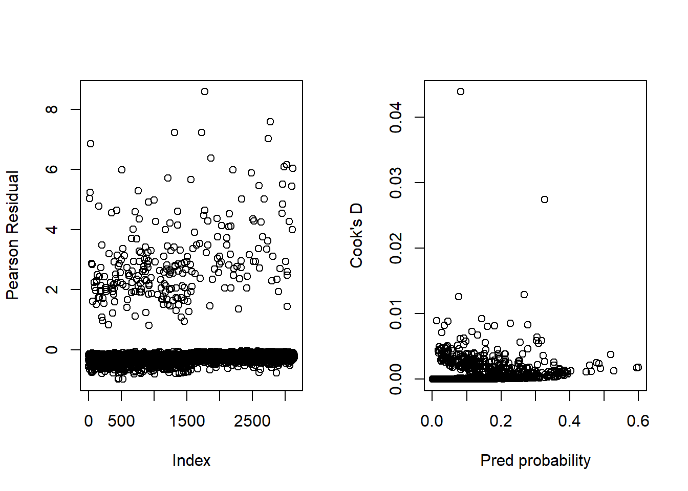
There are different types of useful residual plots we can produce. Firstly we have an index plot displaying the Pearson (or deviance) residual vs the ordered observation number in the dataset. This plot allows us to identify large residuals. Secondly there is the Cook’s distance plotted against the predicted probability. These two plots can be found side-by-side in the figure below, see also p. 175-176 in Vittinghoff et al. (2012). You can also examine other diagnostic tools like leverage and draw other plots e.g. Pearson (or deviance) residuals vs predicted probabilities.
We clearly see the grouping of residuals by CHD status on the left panel but there is no indication that an observation has a residual that is much larger than the others. Note that some of these residuals are well above 2 and that’s perfectly fine. The standardisation carried out in the standard Pearson residuals does not mean that their variance is 1. A similar plot can be produced for the deviance residuals (omitted) and will lead to a similar interpretation. The plot of the Cook’s distance vs the predicted probabilities identifies two observations with a slightly bigger Cook’s distance (CD). We can identify who they are by sorting the data by decreasing CD and printing the top 2-5 observations. The one with the largest CD is patient 10078 with CHD who does not smoke, is very obese (BMI=38.9) and a cholesterol below average (188 mg/dL = 4.86 mmol/L). The next one is patient 12453 who did not have CHD, smokes and has a very high SBP (196). Although these two observations stand out, they are not overly influential on the fit. A case-deletion and refit would lead us to a similar conclusion. Note that you may get different values in Stata but similar looking plots (up to different scaling in the way the Cook’s distance is calculated in the respective pacakages). A lot of other plots can be produced like in linear regression: you can for instance compute the dfbetas (one per parameter) and plot them to identify influential observations or use leverage values again for other plots. There is no real equivalent of residuals-squared versus leverage. Plot of Pearson or deviance residuals versus a particular covariate are not particularly useful to identify remaining structures than the model may not have captured (like a quadratic trend in age). This will be examined using splines - see week 11 material.
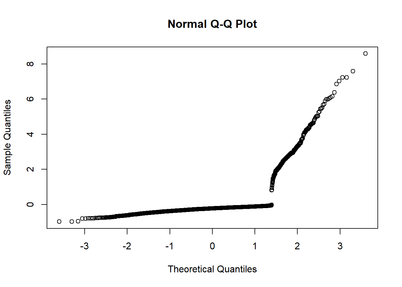
We said earlier that we should not expect the Pearson or deviance residuals to be normally distributed. What happens if we draw a normal probability plot anyway? The figure below displays such a plot and we can clearly see the separation between two groups based on the outcome status and plot is a broken line.
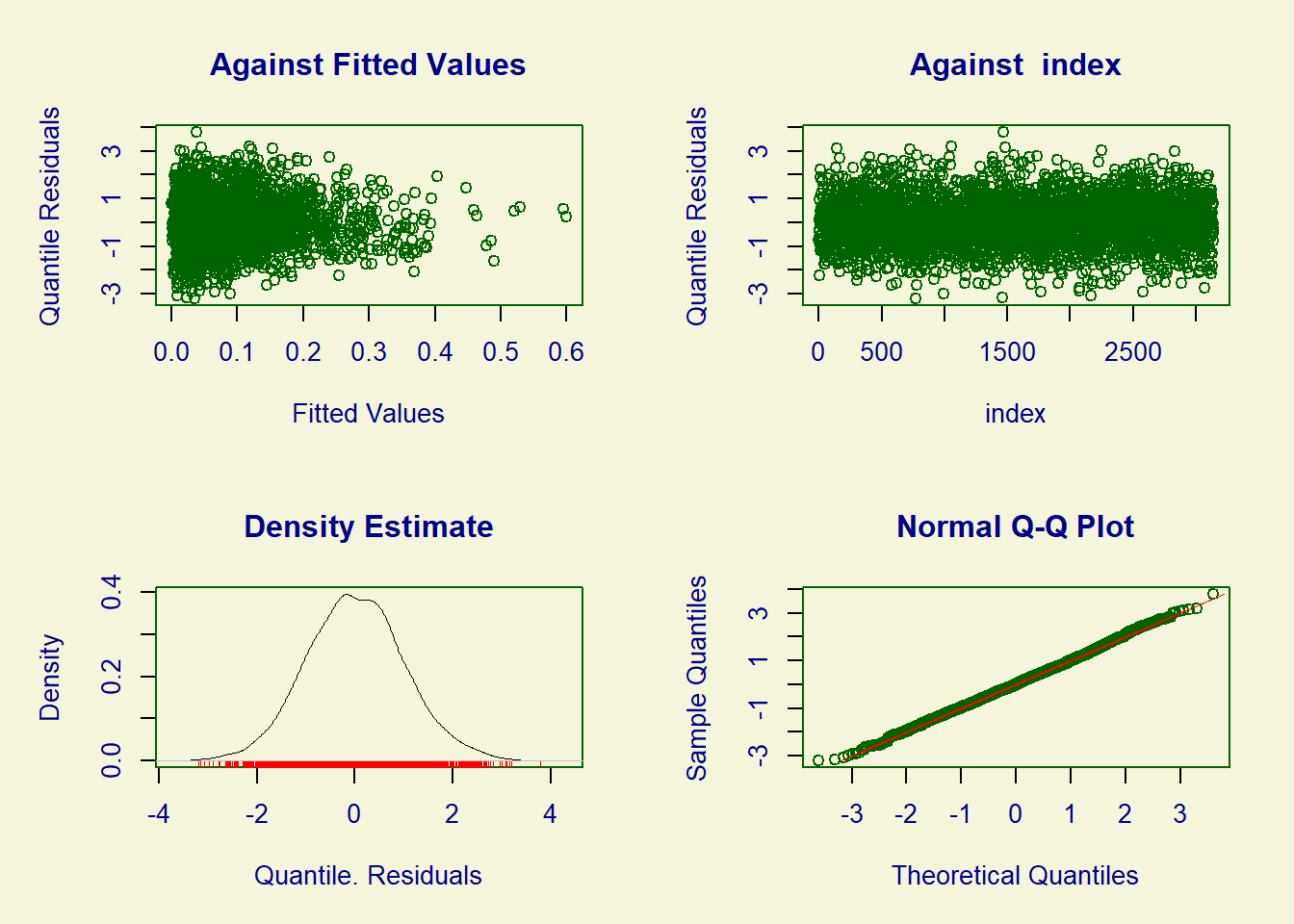
R-users may be able to produce a more meaningful plot using the library gamlss . This library allows you to fit a large variety of models that will be explored in RM2. You can force gamlss to fit a logistic regression model and get the exact same fit as the standard glm command. The code can be found below. The advantage is that a standard plot of the output gives you a much nicer plot of residuals. These resdiduals are called randomised quantile residuals due to Dunn and Smyth (2012). They essentially use randomisation to achieve continuous residuals when the response variable is discrete. Irrespective of the technicality (details to be given in RM2), R produces very nice plots for these residuals.
R code and output
Show the code
par(mfrow=c(1,1))require(gamlss)## Loading required package: gamlss## Warning: package 'gamlss' was built under R version 4.4.3## Loading required package: splines## Loading required package: gamlss.data## ## Attaching package: 'gamlss.data'## The following object is masked from 'package:datasets':## ## sleep## Loading required package: gamlss.dist## Warning: package 'gamlss.dist' was built under R version 4.4.3## Loading required package: nlme## Loading required package: parallel## ********** GAMLSS Version 5.4-22 **********## For more on GAMLSS look at https://www.gamlss.com/## Type gamlssNews() to see new features/changes/bug fixes.out4<-gamlss(chd69 ~ age_10 + chol_50 + sbp_50 + bmi_10 + smoke + dibpat + bmichol + bmisbp, family=BI, data=wcgs2cc)## GAMLSS-RS iteration 1: Global Deviance = 1576.039 ## GAMLSS-RS iteration 2: Global Deviance = 1576.039plot(out4)
## ******************************************************************
##   Summary of the Randomised Quantile Residuals
##                            mean   =  0.01701444
##                        variance   =  0.9914688
##                coef. of skewness  =  0.07237224
##                coef. of kurtosis  =  3.067414
## Filliben correlation coefficient  =  0.9996639
## ******************************************************************
A nice straight QQ plot of this randomised quantile residuals is produced meaning that there are no particular issues in the residuals to be concerned about. R-users can try to run the code given above and first verify that gamlss and glm gave the same fit. The plot command issued right after the fit may however return a completely different figure due to a different implementation in gamlss. To our knowledge, there is no equivalent to this function gamlss in Stata.
The following are the key takeaway messages from this week:
The concept of interaction is similar to the one used in linear regression when expressed on the logit scale. Effect modification is mutiplicative on the odds-ratio scale.
Predicted probabilities of an event and 95% CI can be calculated for any patient’s profile.
Residuals can also be extended (e.g. the Pearson and deviance residuals) but they are not normally distributed.
Other diagnostic tools (e.g. leverage, Cook’s distance) exist and have similar interpretation. They can help identify outliers and influential observations.